1. Study the effects of contrast enhancement histogram equalization and histogram stretching.
2. Study the effects of histogram equalization via HISTEQ function.
3. Utilizing the SUBPLOT function to display images.
4. Study the effects of spatial filtering using IMNOISE, FSPECIAL, and MEDFILT2 functions.
5. Study image noise and how the median and average filters remove noise.
6. Study different methods of edge detection for use on noisy images specifically motion blur, Gaussian noise and filtered Gaussian noise via averaging.
7. Formulate real-world applications which utilize the above functions and concepts.

project2.m contains six parts.

1. IMRESIZE function utilization for image expansion.
2. Contrast stretching using IMADJUST and STRETCHLIM functions.
3. Histogram equalization using HISTEQ function.
4. Data display utilizing SUBPLOT function.
5. Spatial filtering using IMNOISE, FSPECIAL, and MEDFILT2.
6. Edge detection on noisy images using Matlab noise and edge detection functions.

Executing project2.m from Matlab

At the command prompt enter:

>>project2

Results described in order following Methods section above.

Part 1
The original image, saltAndPepper.gif, was spatially expanded 4x in each dimension using bi-cubic interpolation. The IMRESIZE function was utilized to perform the operation.

Figure 1: Original image. (saltAndPepper.gif)

Figure 2: saltAndPepper.gif spatially expanded by 4x. (saltandpepper_bicubic.jpg)

Part 2
This part implements a scheme of contrast stretching.

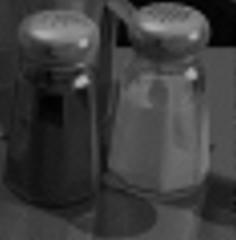
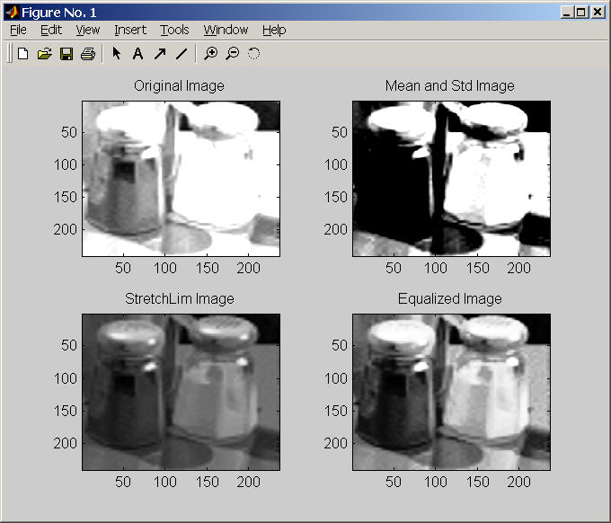
First, the image was intensity scaled such that the lowest intensity had value 0 and the highest intensity had value 255. This was done using the IMADJUST function. It was found by Matlab, that Figure 2's highest intensity value was 180 and the lowest was 0. These values were used in computing the input high and low values for the IMADJUST function. As expected, the image had better contrast due to the better intensity spread of pixels.

Figure 3: Adjusted figure 2 such that the lowest and highest intensities are 0 and 255 respectively. (saltandpepper_imadjust.jpg)

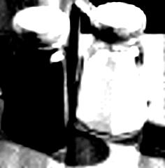
LOW_IN = (mean-(standard deviation)/2)/256 = 0.1790
HIGH_IN =(mean+(standard deviation)/2)/256 = 0.2980

Figure 4: IMADJUST performed on Figure 2 with LOW_IN and HIGH_IN equal to above calculations (saltandpepper_mean.jpg)

The mean was  61.0622 and the standard deviation was 30.4731.

Figure 4 was as expected as the values that were 0.5 sigma (std. dev.) to the right and left of the mean were stretched across the entire spatial domain (0 to 255). Thus, removing some of the intermediate grey values by spreading those pixels across the entire grayscale domain. This would make our image 'highly' black and white as depicted.

Finally, STRETCHLIM was used to compute the tolerance from the IMADJUST function. The lowest intensity was 0.0. The highest intensity was 0.7059. The results are as expected and were similar to those of part a of this section. This is because these two parts perform a similar function on the input image.

Figure 5: STRETCHLIM performed with IMADJUST on Figure 2 (saltandpepper_stretchlim.jpg)

Part 3
Histogram equalization was performed using the HISTEQ function.

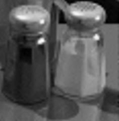
Figure 6: Figure 1 with an equalized histogram (saltandpepper_EqualizedImage.jpg)

Figure 6 was as expected as the image contrast increased.

Part 4

Data display using the SUBPLOT function to plot 4 images (figures).

Figure 7: Plots of images from Part 2. It should be noted that these images were displayed using IMAGE and not IMAGESC. If IMAGESC was used, the original image would be very similar to the StretchLim image due to the nature of the IMAGESC function. (plot1.jpg)

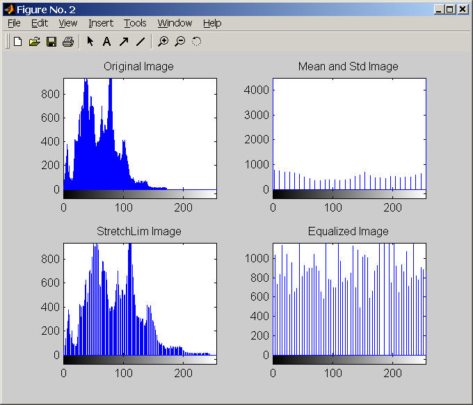
Figure 8: Histograms of the images of Figure 7.(histograms.jpg)

The histograms were as expected by the concepts and methods of part 2.

Part 5
Noise and noise filtering were studied in this section.
Noise was injected into the equalized image. Noises implemented were Gaussian and salt and pepper. Averaging filters and median filters were utilized to study their effects of noise removal.

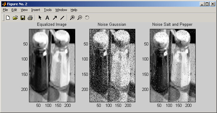
Figure 9: Plot of the original and noisy images. (index.1.jpg)

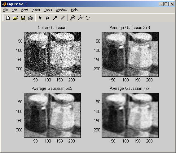
Figure 10: Plot of the Gaussian noisy image and average filtering conducted on that image. (index.2.jpg)

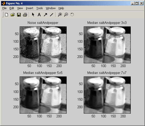
Figure 11: Plot salt and pepper noisy image and median filtering results. (index.3.jpg)

Part 6
Four different types of edge detection were studied. They were: Prewitt, Canny, Roberts, and Sobel.

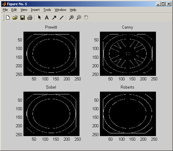
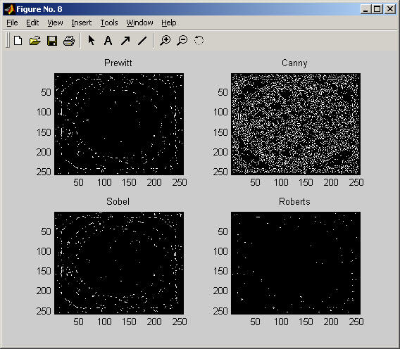
Figure 12: Image used for edge detection analysis (wheel.gif)

Edge detection of all four types was performed on Figure 11. Canny yielded the best results. This was expected as Canny edge detection accounts for regions in an image. Canny yields thin lines for its edges by using non-maximal suppression. Canny also utilizes hysteresis when thresholding.

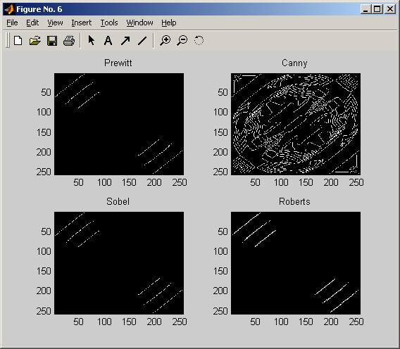
Figure 13: Results of edge detection on Figure 11. Notice Canny had the best results. (index.4.jpg)

Motion blur was applied to Figure 12. Then, the edge detection methods previously used were utilized again on this new image to study their affects in blurry image environments. No method appeared to be useful for real world applications. However, Canny produced the best the results out of the set.

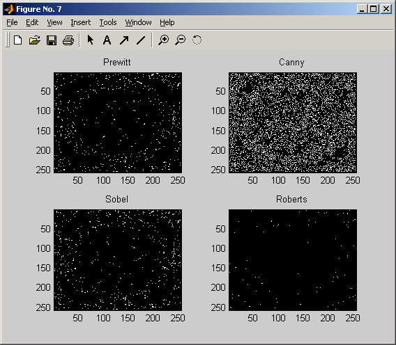
Figure 14: Results of edge detection on a motion blurred Figure 9.  (index.5.jpg)

Gaussian blur was applied to Figure 12. Then, the edge detection methods previously used were utilized again on this new image to study their affects in Gaussian noisy  image environments. No method appeared to be useful for real world applications. This was expected as Gaussian noise corrupts edges and image detail making it difficult to distinguish clear regions in an image.

Figure 15: Results of edge detection on a Gaussian noisy version of Figure 9.  (index.6.jpg)

Gaussian blur was applied to Figure 12. Then, a 3x3 average filter was applied to this image. The edge detection methods previously used were utilized again on this new image to study their affects for averaged filtered Gaussian noisy images. No method appeared to be useful for real world applications. However, Prewitt and Sobel were the most affective out of the set. This was because these filters have a larger mask size than Roberts and thus can show gradient information over a larger area. This is useful because image averaging spreads each pixels information over an area larger than one pixel, in this case a 3x3 area.

Figure 13: Results of edge detection on an 3x3 average filtered  Gaussian noisy version of Figure 12.  (index.7.jpg)

Summary
All results were as expected in the experiment. It should be noted that Canny edge detection works best for non-noisy, non-moving images.

There are many different interpolation methods used in resizing an image. Image enlargement is a common resize method necessary to blow up images in order to see features better. A common interpolation is bi-cubic. It is often used because it weights pixel intensity's to smooth the enlarged image and remove blockiness.

There are many different ways to increase contrast and features of an image. These concepts are inportant for recognition of objects and important features of an image. Histogram equalization is a simple way to increase the contrast of an image. By stretching the pixels 'around' the mean intensity, an image emphasizing the light and dark areas of an image can be realized.

Contrast is usually at its maximum when an image's histogram is uniform, or equalized. Matlab has a function that can take an arbitrary image and make its histogram close uniform. This function is called HISTEQ and is commonly used to increase image contrast.

The SUBPLOT function was used to neatly plot and label output images into one window. This function can be used to easily compare images and label them neatly for public use.

Images always contain some amount of noise. It is often useful to model or simulate different types of noise in order to design filters to remove it or study its effects on other image transformation (eg. edge detection algorithms). There are different types of noises such as Gaussian noise and salt and pepper noise. There are filters that can be applied to an image to try to remove noise. These filters can be average filters or median filters. Average filters are often used to remove Gaussian noise as they help 'smooth' the noise out over the image. Median filters are often used to remove salt and pepper noise as the 'salt' or 'pepper' pixels rarely are ever the median of a pixel neighborhood.

Edge detection is commonly used for object tracking, recognition, etc. There are many different algorithms to detect edges. Each has their advantages and disadvantages. We studied Canny, Roberts, Sobel, and Prewitt edge detection masks. Noise can affect the results of these edge detection algorithms. In environments where edge detection is often used, motion blur is often a problem. For non noisy images, Canny appeared to work the best. In noisy environments, Prewitt or Sobel yeilds best results after an average filter is applied. However, these results appeared to not be very useful in real-world applications. In motion blurry environments, Canny seemed to be the most affective of the four filters. However, the results it produced would be hard to utilize in a real world enviroment.