CSE/EE 485: Digital Image Processing IComputer Project Report # : Project 4Inverse FilteringGroup #4: Isaac Gerg, Pushkar DurveDate: November 18, 2003 |
||||||||||||||
|
|
||||||||||||||
| A. |
Objectives
|
|||||||||||||
| B. |
Methods There is one 'M' file for this project. project4.m contains six parts.
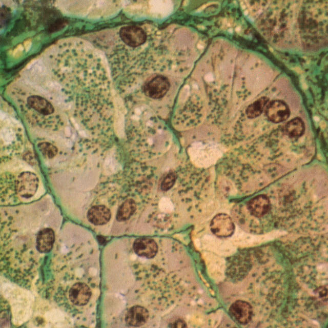
1. Conversion of RGB image to gray level. Executing project4.m from Matlab At the command prompt enter:
|
|||||||||||||
| C. |
Results Image file names in parentheses. Results described in order following Methods section above.
Part 1
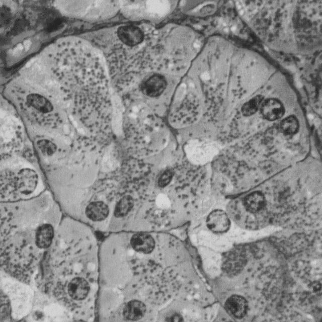
Part 2
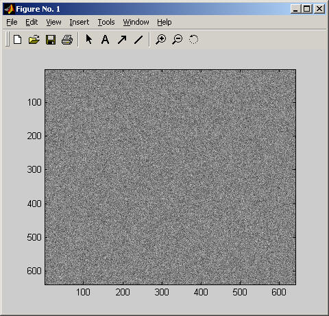
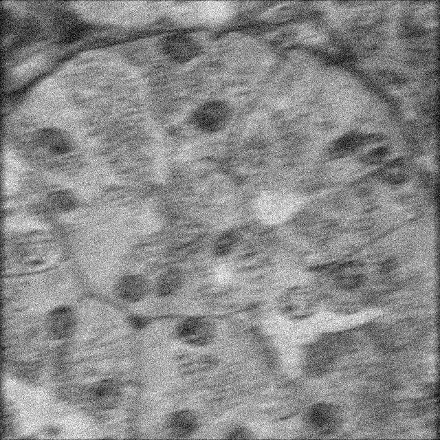
Figure 3: The Gaussian Noise Matrix scaled by intensity to 0 and 1 respectively.(index.4.jpg) Part 3 A PSF was created using the FSPECIAL function using the 'motion' parameter. The image in Figure 2 was then motion blurred using this PSF and the IMFILTER function. Then, Gaussian noise was added with the IMADD function and the Gaussians Noise Matrix. The output of this operation on Figure 2 is shown in Figure 4.
Figure 4: Degraded image of Figure 2 using motion blur and Gaussian noise (tissue1_blur_and_noise.jpg) Part 4 The Noise to Signal Power Ratio was computed using the following equations:
The equations were calculated for the image of Figure 2 and the image of Figure 3. The powers were then divided to get the Noise to Signal Power Ratio.
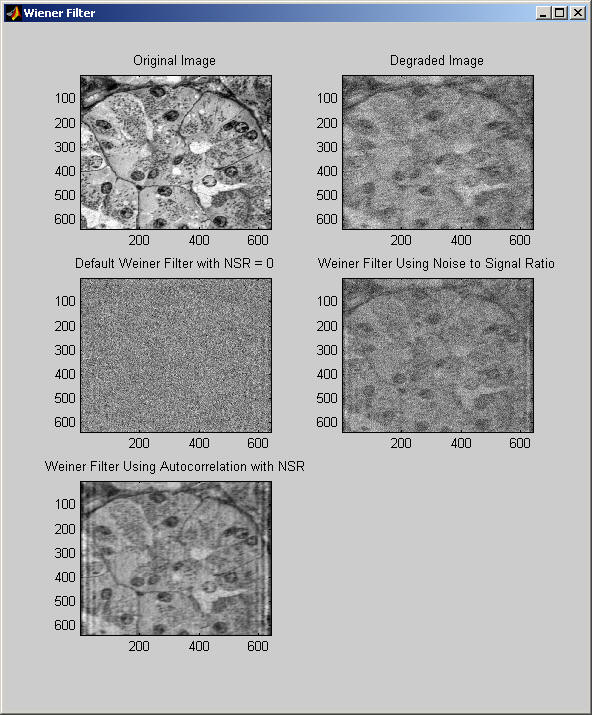
Part 5 Two autocorrelation matrices were computed using the IFFT2 command and the REAL command. This returned the real part of the inverse fast Fourier transforms of the spectrums of figure 2 and figure 3. These matrices are used in the inverse filtering of Figure 4 later in the experiment. Part 6 The DECONVWNR function was used to perform Wiener filtering on Figure 3. There are many different parameters that can be used with this type of inverse filtering. Figure 5 shows these parameters being applied. Notice that the more information we give the filtering function, the better the results.
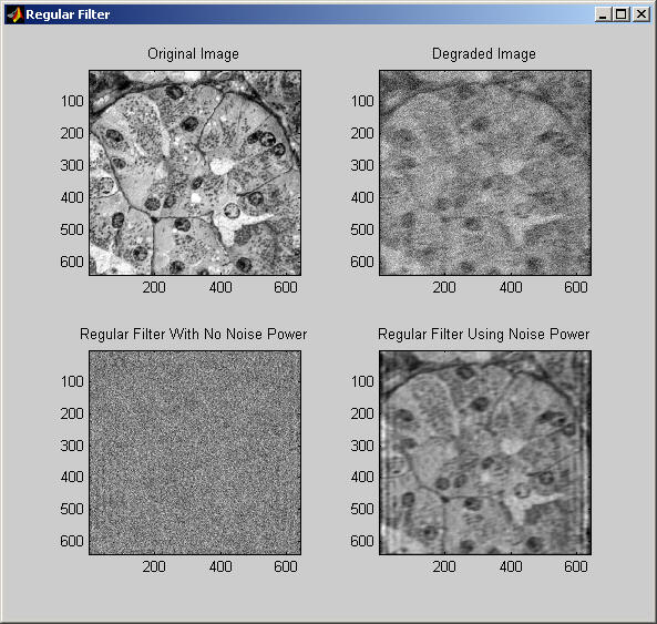
Figure 5: Results of Wiener filtering using different parameters. (index.1.jpg) Part 7 The DECONVREG function was used to perform Regularized filtering on Figure 3. There are many different parameters that can be used with this type of inverse filtering. Figure 6 shows these parameters being applied. Notice that the more information we give the filtering function, the better the results. With no noise power information, the image is heavily degraded. This is because the filter looks at the extra noise in the image as part of some degradation function (blurring possibly) and not as additive noise.
Figure 6: Results of Regularized filtering using different parameters. (index.2.jpg)
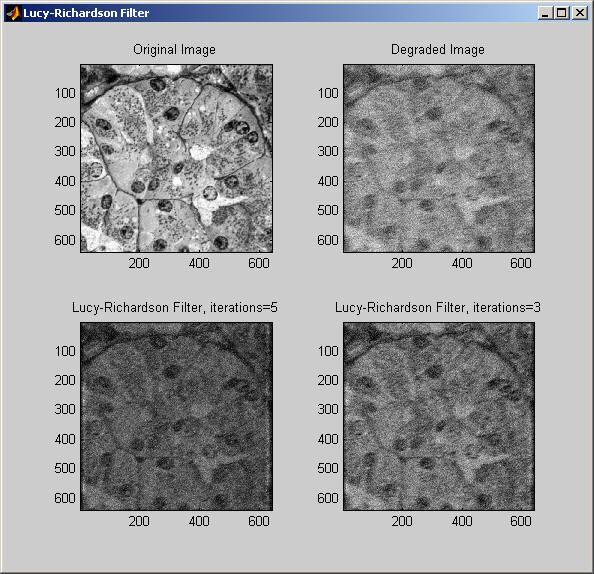
Part 8 The DECONVLUCY function was used to perform Lucy-Richardson filtering on Figure 3. There are many different parameters that can be used with this type of inverse filtering. Figure 7 shows these parameters being applied. Notice that as the number of iteration we performed on the image increased, the better quality output image was realized. This filter is particularly interesting as it could remove much of the blur and still leave the noise in the image. This was not found with the two previous filters.
Figure 7: Results of Lucy-Richardson filtering using different parameters. (index.3.jpg) CPU Time The CPU time used to conduct this experiment was:
|
|||||||||||||
| D. |
Conclusions Often the color information if an image is irrelevant to analysis. When this is the case, a color image is often converted to grayscale to speed up computation. In real life, you don't know what the PSF is. You guess the PSF based on camera parameter or other system characteristics. It can be found even though experiment. However, the PSF is usually a model as its very complex to determine an exact PSF. Noise in am image is commonly modeled as Gaussian. The noise to image power ratio is good measure of how much noise is in an image. This information, along with the noise power, can be used in the inverse filtering process to realize a much less degraded image. As expected the more information you add to the inverse filtering process, the better the output. Autocorrelation matrices are often used in inverse filtering. The come from noise and blur information about the image. This information expressed as a correlation is a convenient way to implement it into an inverse filter. With no noise information, the Wiener and Regularized filters do a poor job at realizing the original, non degraded, image. However, the Lucy-Richardson filter works really good, despite having no information about the noise in the image. With noise information, the Wiener and Regularized filters do a great job at restoring the image. However, the Wiener filter is much better at the blur than the Regularized filter. Despite having no noise information, the Lucy-Richardson filter performs rather well at removing the degradation from the PSF (blur in the case) but not the noise. The chart below (Figure 8) summarizes what configuration work best with what filter assuming you have a good PSF.
|
|||||||||||||
| E. |
Appendix project4.m source code.
|
|||||||||||||
|
|
||||||||||||||