1. Study JPEG compression for images and the effects of lossy compression
2. Study MPEG compression for movies and the effects of lossy compression.
3. Study mathematical morphology and its uses for object extraction.
4. Implement iterative scene and image operations via MATLAB scripting.
5. Formulate real-world applications which utilize the above functions and concepts.

There is one 'M' file for this project.

project5.m contains four parts.

1.  JPEG compression analysis
2.  MPEG compression analysis
3.  MPEG playback via MATLAB routine.
4.  Cell (organism) extraction via Mathematical morphology

Executing project5.m from Matlab

At the command prompt enter:

>>project5

Results

Results described in order following Methods section above.

Part 1
In this section we studied how multiplicatively scaling the quantization matrix changes the compression ration and image quality. The discrete cosine transfer (DCT) was performed on the image for an 8x8 block. The matrix was then quantized using that quantifier. Next we dequantized the image and performed the inverse DCT to get back our original image. The differences between the original image and the one we computed via DCT and quantization methods were compared. There are differences in the images as expected as lossy compression removes some information from the image when performing compression.

Figure 1: The original and compressed images along with the absolute difference between the images, the Error Matrix.

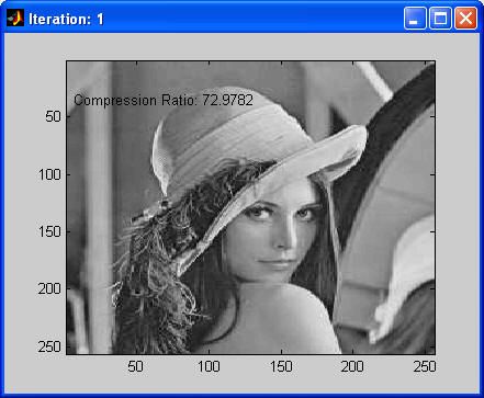
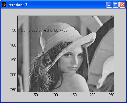
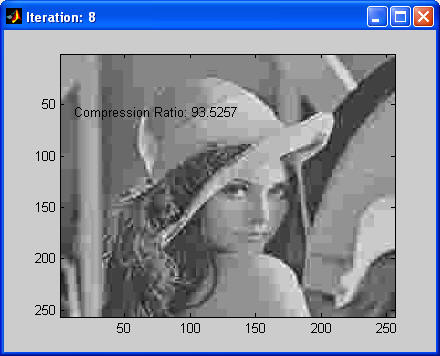
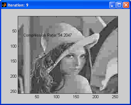
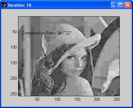
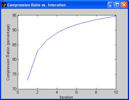
We then created a loop from 1 to 10 and ran the compression algorithm described above on the original image. With each iteration, we multiplicatively scaled the quantization matrix by the loop index to see its effects on compression. You can see that as the iteration get higher, the compression ration increases and image quality is lost. The factor used to adjust the quantization matrix is called the Q-Factor.

Below is a plot of the compression ration versus iteration.

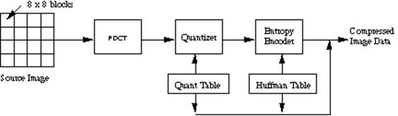
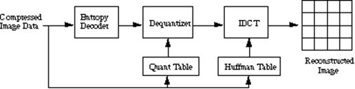
JPEG Encoder Block Diagram  

   JPEG Decoder Block Diagram

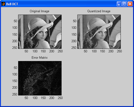
The DCT-based encoder can be thought of as essentially compression of a stream of 8x8 blocks of image samples. Each 8x8 block makes its way through each processing step, and yields output in compressed form into the data stream. Because adjacent image pixels are highly correlated, the `forward' DCT (FDCT) processing step lays the foundation for achieving data compression by concentrating most of the signal in the lower spatial frequencies. For a typical 8x8 sample block from a typical source image, most of the spatial frequencies have zero or near-zero amplitude and need not be encoded. In principle, the DCT introduces no loss to the source image samples; it merely transforms them to a domain in which they can be more efficiently encoded.

After output from the FDCT, each of the 64 DCT coefficients is uniformly quantized in conjunction with a carefully designed 64-element Quantization Table. At the decoder, the quantized values are multiplied by the corresponding QT elements to recover the original unquantized values. After quantization, all of the quantized coefficients are ordered into the "zig-zag" sequence. This ordering helps to facilitate entropy encoding by placing low-frequency non-zero coefficients before high-frequency coefficients. The DC coefficient, which contains a significant fraction of the total image energy, is differentially encoded.

Part 2
In this part we converted a 4D matrix to a 3D matrix via the RESHAPE function. We also read in the matrix, displayed each frame and then formed a movie matrix, M, and then wrote this movie to disk in MPEG format.

Part 3
The assembled MPEG movie was read into MATLAB and played back via the MOVIE function.

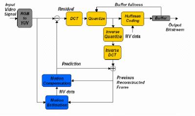
MPEG Encoder Block Diagram  

Figure 6: MPEG Encoder

On the left side the original image can be seen, which is represented by its luminance signal and its two chrominance signal components. A motion compensated image is then subtracted from the original image. In the case that the original image is a B- or P-picture, the motion compensated image is an estimation of the original image. In the case, that the original image is an I-Picture, one can assume a motion compensated image with all pixel values being equal to zero. 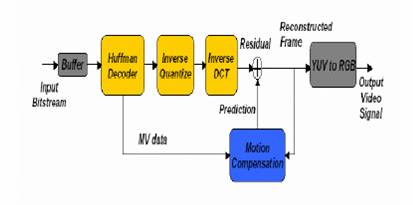The motion compensated image comes from the motion compensation box.

A two-dimensional DCT coding is applied to the resulting difference image (box "DCT") and its spectral coefficients are quantized in the box "Q". After a sorting the quantized spectral coefficients are entropy encoded and the codewords are written into a buffer memory. The MPEG bitstream is taken out of this buffer.

The type of the picture and the amount of data in the buffer control the quantization. If the amount of data in the buffer increases, the quantization will become coarser. If the amount of data decreases, the quantization will become finer.

The motion compensation needs the image, which is reconstructed from the quantized spectral coefficients. So an "inverse quantization" (box "Q^-1") takes place and the inverse DCT (box "DCT^-1") creates the reconstructed image, which will be fed into the motion compensation. The reconstructed image is equal to the image, which will be found at the receiver side, if no transmission errors have occurred.
 

MPEG Decode Block Diagram  

Figure 7: MPEG Decoder

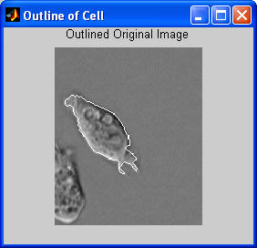
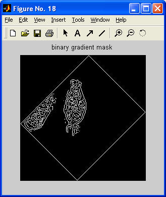
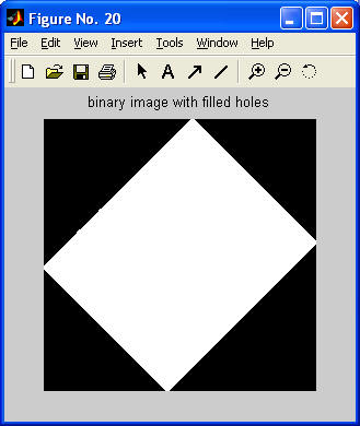
The MPEG decoder reads the data out of sequence, does the frame recomposition taking into account the stored motion information and differential frames present, and then reorders the frames into correct time sequence before outputting them.

Part 4

This part used the image segmentation algorithm and did a good on the non-rotated and 90 degrees images.  This can be seen in Figure 8 and Figure 9.  The algorithm did not perform too good on 45 degree rotated source as seen in Figure 10.

The reason the Algorithm 3 of Part 10 did not work was because a command was done to fill all holes in the object.  Edge detection detected the bouding in the 45 deg. rotated image and bounded it, thus killing the object.  

Figure 8: Outlined Original Image


Figure 9: Binary Gradient Mask


Figure 10: Binary Image with Filled Holes

Summary
All results were as expected in the experiment.

Uncompressed multimedia (graphics) data requires considerable storage capacity and transmission bandwidth. Despite rapid progress in mass-storage density, processor speeds, and digital communication system performance, demand for data storage capacity and data-transmission bandwidth continues to outstrip the capabilities of available technologies. The recent growth of data intensive multimedia-based web applications have not only sustained the need for more efficient ways to encode signals and images but have made compression of such signals central to storage and communication technology.

A common characteristic of most images is that the neighboring pixels are correlated and therefore contain redundant information. The foremost task then is to find less correlated representation of the image. Two fundamental components of compression are redundancy and irrelevancy reduction. Redundancy reduction aims at removing duplication from the signal source (image/video).  In general, three types of redundancy can be identified:

• Spatial Redundancy or correlation between neighboring pixel values.

• Spectral Redundancy or correlation between different color planes or spectral bands.

• Temporal Redundancy or correlation between adjacent frames in a sequence of images (in video applications).

Image compression aims at reducing the number of bits needed to represent an image by removing the spatial and spectral redundancies as much as possible.

Mathematical Morphology is the analysis of signals in terms of shape. This simply means that morphology works by changing the shape of objects contained within the signal.

There are many more applications that morphology can be applied to. Morphology has been widely researched for use in image and video processing.

MRI Movie