1. Implement image matrix transformations including translation and rotation.
2. Implement two different interpolation methods including nearest neighborhood and linear.
3. Study the effects of image rotation and different interpolation methods.
4. Become familiar with the camera on whitemouse.
5. Become familiar with Matlab programming and the Image Processing Toolbox.

project1.m contains six parts.

1. Creation of Translation Matrix, T.
2. Creation of Rotation Matrix, R.
3. Creation of transformation matrix, M.
4. Implement image transformation using matrix M.
5. Performed Nearest Neighbor Interpolation with transformation matrix, M.
6. Performed Linear Interpolation with transformation matrix, M.
 

Executing project1.m from Matlab

At the command prompt enter:

>>project1

Results described in order following Methods section above.

Figure 1: Output of the original image, nearest neighborhood interpolation image, and linear interpolation image (Order is left to right respectively). (images.jpg)

Part 1
Created a translation matrix, T. The image was translated 16 pixels in the positive X direction and 16 pixels in the positive Y direction.

Part 2
Created rotation matrix, R. The image was rotated 15 degrees counter-clockwise. 15 degrees was changed into radians for our rotation matrix.

Part 3
Created transformation matrix, M.
M = (R) (T)

Part 4
Implemented image transformation using matrix, M. Created a loop which iterates through every pixel in the output image. The output pixel's intensity level is realized by mapping back to the correct input pixel using the inverse of matrix M.

Part 5
Performed nearest neighborhood interpolation. If integer coordinates could not be mapped back to the input image, the coordinates were rounded to select the proper pixel. The Matlab function ROUND was utilized.

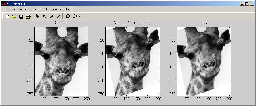
Based on observation, the edges in the image were not smoothed. There were some slightly jagged lines that were noticed in the rotated image that were not present in the original image.

Part 6
Performed linear interpolation. If integer coordinates could not be mapped back to the input image, the correct output pixel intensity was realized by performing a weighted average of pixels near the real numbered coordinate.

OutputImage(x', y') = (1-a)(1-b) (InputImage(r,c)) + (a)(1-b)(InputImage(r+1, c)) + (b)(1-a)(InputImage(r, c+1)) + (a)(b)(InputImage(r+1, c+1))

r = FLOOR(x), c = FLOOR(y), a = x - r, b = y - c

where FLOOR is the Matlab floor function.

Based on observation, the edges in the image were noticeably smoother than what was observed using nearest neighborhood interpolations. This was expected as a weighted pixel intensity was used when integer coordinates were not realized in calculation.

Summary
All results were as expected in the experiment. The outputs are in Figure 1.

Using homogenous coordinates, one can create matrix transformations simply by multiplying matrices together.

There are many different methods to scale, rotate, etc. an image. Due to the discreteness of our image matrix, some visual information may be misinterpreted. This can be corrected by utilizing different interpolation methods.

Nearest neighborhood interpolation yields a suitable image. However, it is not as refined as an image created using linear interpolation. Linear interpolation would be used in any type of image rotation where smoothness of the image must be preserved. Translation and rotation functions are used commonly in elementary image editing.

Source Code

project1.m source code.

% ----------------------------------------------------------------------
% - CSE 486
% - Project 1
% - Group 8
% - idg101, adi102, jlm522
% ----------------------------------------------------------------------

% Read in image.
I = imread('giraffe.jpg', 'jpg');

% Translate image 16 pixels along X and Y axis.
T = [ 1 0 0 -16;
0 1 0 16;
0 0 1 0;
0 0 0 1];

% Rotate image ccw 15 degrees.
angle = (-15*pi/180);
R = [cos(angle) sin(angle) 0 0;
-sin(angle) cos(angle) 0 0;
0 0 1 0;
0 0 0 1];

% Create ouput image.
M = R*T;
for x_index = -127:128
for y_index = -127:128
OutputVector = inv(M) * [x_index; y_index; 0; 1];
x = OutputVector(1);
y = OutputVector(2);

% Nearest Neighborhood Interpolation (nni)
x_nni = round(x);
y_nni = round(y);

% Linear Interpolation (li)
r = floor(x);
c = floor(y);
a = x - r; b = y -c;

% Ensure coordinates of I are valid.
if (x_nni > 128 | x_nni < -127 | y_nni > 128 | y_nni < -127)
O_nni(x_index + 128, y_index + 128) = 255;
else
% Nearest Neighborhood Interpolation
O_nni(x_index + 128, y_index + 128) = I(x_nni + 128, y_nni + 128);
end

% Linear Interpolation
% Ensure coordinates of I are valid.
if (r > 128 | r < -127 | c > 128 | c < -127)
point_north = 255;
else
point_north = double(I(r + 128, c + 128));
end
if (r + 1 > 128 | r + 1 < -127 | c > 128 | c < -127)
point_east = 255;
else
point_east = double(I(r + 1 + 128, c + 128));
end
if (r > 128 | r < -127 | c + 1 > 128 | c + 1 < -127)
point_south = 255;
else
point_south = double(I(r + 128, c + 1 + 128));
end
if (r + 1 > 128 | r + 1 < -127 | c + 1 > 128 | c + 1 < -127)
point_west = 255;
else
point_west = double(I(r + 1 + 128, c + 1 + 128));
end
O_li(x_index + 128, y_index + 128) = (1-a)*(1-b)*point_north + a*(1-b)*point_east + b*(1-a)*point_south + a*b*point_west;
end
end

% Display and title output.
colormap('gray');
subplot (1,3,1);
imagesc (I);
title('Original');
subplot (1,3,2);
imagesc (O_nni);
title('Nearest Neighborhood')
subplot (1,3,3);
imagesc (O_li);
title('Linear');

Time Management
Each member of the group spent four hours working on this project.