A.

 Objectives

1. Become familiar with reading and writing images.
2. Become familiar with theory and application of basic morphological operations.
3. Study the effect of morphological spatial filtering when applied to binary images.
4. Study the applications of border detection of binary object.
5. Study the effects of shape-based filtering with binary images.
6. Formulate real-world applications which utilize the above functions and concepts.

B.

Methods

One top level MATLAB 'M-file' was used to implement the experiment for this project. The top level 'M-file' performs calls to several functions in order to carry out the required operation. The top level 'M-file' is pj1.m.

pj1.m contains 3 parts.

1. Basic image reading and writing and an application of mean filtering.
2. Binary image processing using basic morphological operations including opening and closing.
3. Shape based filtering using the previously studied operations from above.

Executing pj1.m from MATLAB

At the command prompt type:

>>pj1

C.

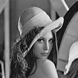
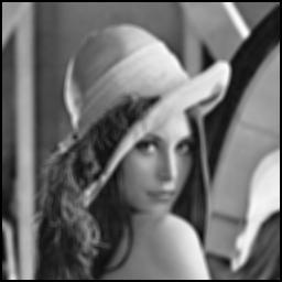
Results

The project was completed in MATLAB using custom functions written to meet the specifications of the project. Results are presented by showing initial images and images that are produced by the algorithm being discussed. In each figure caption image filenames are in parentheses. The results presented in this section are given in the same order delineated in the Methods Section.

Part 1

The original image (Figure 1) was filtered using a 5x5 average filter. The output of this operation is Figure 2. Notice that the output has a small black border as our implementation sets a pixel to zero if there is insufficient local knowledge to perform the operation correctly. No mirroring or padding is performed. The result in figure 2 is blurry relative to the original image.  This result is expected for a mean filter. The blurriness results from the low-pass frequence response of the mean filter which removes sharp intensity transitions.  While all of these effects are interesting, the key result from this part of the project is the successful read in and write out of an image.

Figure 1: The original image. (lenna.gif)	Figure 2: The output of average filtering. (Lenna_5x5_averaged.jpg)

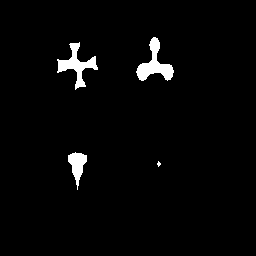
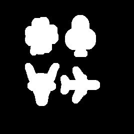
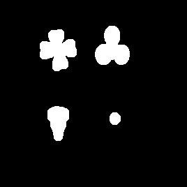
Part 2

In this section we performed basic binary morphological operations on several images. The operations performed were prescibed by the project description. This part has three subparts, A, B and C enumerated below.

Part 2.A

The following operations were performed on Figure 3: erosion, dilation, opening, and closing. Note, the structuring element was originally a 5x5 circle and was dilated with itself 2 times before the operations were performed. Dilation of a structuring element results a larger structuring element with similar properties of the original. For example, B dialated with iteslf once is 2B and is shown below as well as the original 5x5 circle structuring element.

B = 0 1 1 1 0         2B = 0 0 1 1 1 1 1 0 0         3B = 0 0 0 1 1 1 1 1 1 1 0 0 0
    1 1 1 1 1              0 1 1 1 1 1 1 1 0              0 0 1 1 1 1 1 1 1 1 1 0 0
    1 1 1 1 1              1 1 1 1 1 1 1 1 1              0 1 1 1 1 1 1 1 1 1 1 1 0
    1 1 1 1 1              1 1 1 1 1 1 1 1 1              1 1 1 1 1 1 1 1 1 1 1 1 1
    0 1 1 1 0              1 1 1 1 1 1 1 1 1              1 1 1 1 1 1 1 1 1 1 1 1 1
                           1 1 1 1 1 1 1 1 1              1 1 1 1 1 1 1 1 1 1 1 1 1
                           1 1 1 1 1 1 1 1 1              1 1 1 1 1 1 1 1 1 1 1 1 1
                           0 1 1 1 1 1 1 1 0              1 1 1 1 1 1 1 1 1 1 1 1 1
                           0 0 1 1 1 1 1 0 0              1 1 1 1 1 1 1 1 1 1 1 1 1
                           0 0 1 1 1 1 1 0 0              1 1 1 1 1 1 1 1 1 1 1 1 1
                                                          1 1 1 1 1 1 1 1 1 1 1 1 1
                                                          0 1 1 1 1 1 1 1 1 1 1 1 0
                                                          0 0 1 1 1 1 1 1 1 1 1 0 0
                                                          0 0 0 1 1 1 1 1 1 1 0 0 0


Note that 2B is 9x9, which is reasonable since dilation will add two new elements to each of the four sides of the structuring element.  Thus each dimension has a net gain of four elements resulting in the new dimensionality. Also notice the increasing roundness of the courners. Similar results are found for 3B.

In the figure captions below, X refers to the image (Figure 3) and 3B refers to the structuring element shown above.

Figure 3: Original image (match1.gif)
Figure 4: X eroded by 3B. (X_erosion_3B.png);
Figure 5: X dilated by 3B. (X_dilation_3B.png)
Figure 6: X opened by 3B. (X_open_3B.png)
Figure 7: X closed by 3B. (X_close_3B.png)

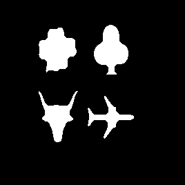
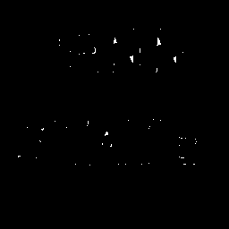
From these results it is clear that dilation expands an object while erosion shrinks it. Expand and shrink are loose terms, but the results demonstrate their meaning. For example, note in Figure 4 that erosion by the large SE 3B has resulted near obliteration of all objects in the image while in Figure 5 dilation by the same SE has distorted the clover to the point that it is almost unrecognizable. Open and close operators attempt to nearly perserve the area of the original objects. The can be seen in be particularly true for closing shown in Figure 7, but with the large SE employed in this experiment the opening operation depicted in Figure 6 has removed more than just details, particularly in the case of the airplane.

Part 2.B

The procedure in this subsection attempts to find the border of arbitrary shapes.  The original image, Figure 8, contains text. The key operation employed in this procedure is set difference. The results clearly demonstrate the expanding effects of dilation and shrinking effects of erosion.

The following morphological operations were performed on Figure 8:

X1 = X-erosion(X,B)

X2  = dilation(X,B)-X

X3 = erosion(dilation(X,B)-erosion(X,B), B)

As above, in X is the original image in Figure 8 and B is the original 5x5 structuring element given in Part 2.A.

Figure 8: Original image X (penn256.gif)
Figure 9: X1 (X1.png)
Figure 10: X2 (X2.png)
Figure 11: X3 (X3.png)

It is obviously quite simple to obtain the outline of an object simply using erosion or dilation.  The choice of operator depends on how one defines the desired outline.  Note that in Figure 9 the outer edge of the outline is the original outer edge of the text characters while in Figure 10 the inner edge of the outline is the original outer edge of the text characters.  This clearly demonstrates the difference between erosion and dilation.  Note that in both cases the width of the remaining outline is two pixels based on the structuring element used (two pixels is the "radius" of the SE employed, the number of pixels from the origin of the SE to the edge). The result from operation X3 is not useful for border detection.

Part 2.C

In this section, proposition 6.7.4 from Nonlinear Digital Filters by Pitas and Venetsanopoulos is demonstrated.  The propositions holds that the the open-close operator by a structuring element of size v+1 is the same as performing a median function with a window of size 2v+1 where v is any integer. The open-close operation is defined as:

close(open(X,2B), 2B)

where X is the original image (Figure 12) and the structuring elements B and 2B are as shown:

B = 1       2B = 1
    1            1
    1            1
                 1
                 1


Since 2B has a size of 5, v=4.  Thus the window A must have size 9.

Figure 12: The original image (X) (bear.gif)
Figure 13: open-close of X (2c.png)
Figure 14: median of Figure 13 (2c_median.png)
Figure 15: Set difference of Figures 13 and 14. (2c_difference.png)

The result of the ope-close operation is shown in Figure 13. Comparision to the original image shows that the few small white "noise" pixels are removed and that some details are filled in while others are removed though the effect is minimal because the SE is relatively small. The output of the median filter, shown in Figure 14, looks identical to the result in Figure 13. The identity of the two is easily verified by taking the set difference of the two, which is shown in Figure 15. The set difference result is completely black (all pixels are zero, indicating there was no difference) which proves that the operations are equivalent.

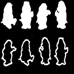
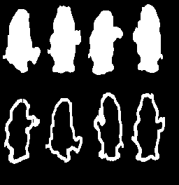
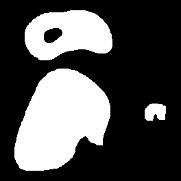
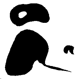
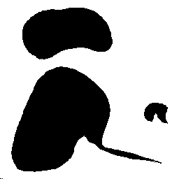
Part 3

The last part of this project is an experiment with shape based filtering. The goal of shape based filtering varies, in this case we focus on the removal of appendages and cavities. The process of conditional dilation is also explored.

Part 3.A

In this section we investigate appendage removal while otherwise attempting to maintain each object's general shape. Several  iterations of erosion on the original image, shown in Figure 16, were performed in order to remove the unwanted appendage. We found it took four erosions to obtain satisfactory results. Each successive erosion to this limit is shown below. The structuring element used for the erosion was a 3x3 square:

B = 1 1 1
    1 1 1
    1 1 1



Figure 16: Original image with unwanted appendage, the tail of the largest object. (TheThreeShapes.gif)
Figure 17: One erosion performed. (3erosion1.png)
Figure 18: Two erosions performed. (3erosion2.png)
Figure 19: Three erosions performed. (3erosion3.png)
Figure 20: Four erosions performed. (3erosion4.png)

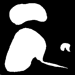
As the iterations progress the objects are increasingly reduced in size. Clearly the appendage on the large object, which we desire to remove is wider than two pixels, though most of it seem to be more narrow than four pixels as three iterations almost completely removes it. Notice that by the 4th iteration, the tail is completely removed from the largest object and the image. Then, to obtain the objects back as best we can, we performed conditional dilation. After each dilation of Figure 20, we checked with set difference to determine if the output was best matched with the original image, Figure16. We the same 3x3 square as the dilation structuring element.

Figure 21: Figure 20 after 1 dilation. (3dialtion1.png)
Figure 22: Figure 20 after 2 dilations. (3dialtion2.png)
Figure 23: Figure 20 after 3 dilations. (3dialtion3.png)
Figure 24: Figure 20 after 4 dilations. (3dialtion4.png)
Figure 25: The set difference of Figure 24 with Figure 16 (3difference.png)

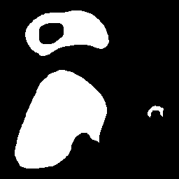
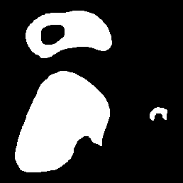
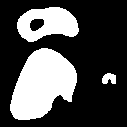
As each dilation is performed the objects get closer to their original size. It makes sense that four successive dilations would lead to approximately the same size objects, but this hypothesis is easly checked with a set difference between the final result, shown in Figure 24, and the original image, shown in Figure 16.  This set difference is shown in Figure 25. The objects present in the set difference represent what was removed from the original objects after four successive erosions followed by four successive dilations.  The goal is to minimize what is removed from the main part of the objects while maximizing the removal of the large appendage on the largest object. The results are positive, as the appendage is the most significant thing removed and the remaining differences are relatively minor.

Part 3.B

Figure 26: Original Image (TheThreeShapes.gif)
Figure 27: X complemented (difference_image.png)
Figure 28: X complemented with cavity deleted (complement_with_no_cavities.png)
Figure 29: X with no cavities (no_cavities.png)

The first step was to compliment the original image. The compliment is shown in Figure 27.  Then all objects but the largest is deleted. Note that there are only two objects in the complement -- what was the background in the original image and what was the cavity that we want to deleted. The latter is deleted resulting in the image shown in Figure 28.  Finally, another complement is performed and the final result, in Figure 29, is the original image without the cavity.

Summary

The results presented here are relatively straight forward. All outcomes achieved were as expected in each experiment, as we were able to predict what we should see and explain each result. The basic morphological operations are demonstrated, however, a result of great significance (other than the completion of our first 585 project) was not achieved.

D.

Conclusions

MATLAB has tools that allow for easy access to image reading and writing. It has convenient method for manipulation grayscale image matrices.

The choice of structuring element has a tremendous impact on the result of morphological operators.  The structuring element must be carefully chosen to meet the specifications of a particular task. An inappropriate structuring element at even one stage in a sequence a morphological operators can obliterate desired features.

Binary image processing can be a useful tool in border detection in binary images. It is also useful for smoothing masks such as those in object detection and extraction.  Sometimes, other non-common operations will perform the same function as a morphological operation as in the case of the median filter and open-close. In these cases, there are often incidents where there operations are idempotent.

Repetitive dilations of a structuring element are useful in enlarging the element but maintaining some its characteristics on a binary image.

Morphological operations are useful to remove unwanted features from an image or mask. These can include appendages and cavities. These removals are often achieved through numerous erosions or dilations. Then, the large objects, blobs, can be restored through numerous dilations. These operations can be combined to quickly remove unwanted noise as in the case with object tracking or masking.

E.

Appendix

This appendix contains the source code for our project. The code is shown below in a way that reflects the hierarchy of dependancies. Please refer to the comments at the top of each function for a complete description.

• pj1.m
  • dilation.m
  • erosion.m
    • erode.m
  • imavgfilter.m
  • median.m
    • med.m
      • rowcat.m
  • setdifference.m