A.

 Objectives

1. Become familiar with conditional morphological operations such as conditional dilation.
2. Learn to appropriately apply conditional operations to images.
3. Study and implement object extraction / connected components using conditional dilation (iterative scheme).
4. Study the the pecstrum function and learn how to interpret pecstrum functions of an object.
5. Explore the process of identifying objects using morphological operators.
6. Use morphological operators to perform skeletonization
7. Evaluate the performance of reconstruction from morphological skeletons
8. Formulate real-world applications which utilize the above functions and concepts.

B.

Methods

The experiment was written in terms of many MATLAB functions with no single script used to execute the entire experiment.  Each function is described below.

findObjects.m  (findObject function)

The function finds all the objects in a binary image, writes out each object to a separate file, computes the pecstrum of each object, writes out the pecstrum to a file, and finally return an image of the original image with the objects isolated and labeled by shades of gray.

SK.m (SK function)

The SK function finds a morphological skeleton using Maragos' serial decomposition documented in
Pitas and Venetsanopoulos (P&V). It returns the skeleton of the input image.

skeleton.m

This M-file serves as the driver to compute a skeletonization of an image.

Executing the functions from MATLAB

Please see the associated help with function. At the command prompt type:

>>help functionname

C.

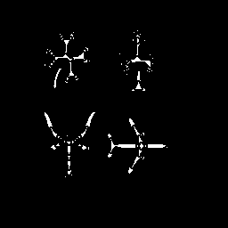
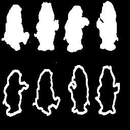
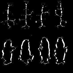
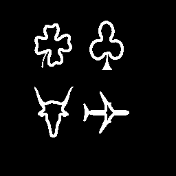
Results

The project was completed in MATLAB using custom functions written to meet the specifications of the project. Results are presented by showing initial images and images that are produced by the algorithm being discussed. In each figure caption image filenames are in parentheses.  The image displayed in this report may be scaled in the document in order to enhance readability.  However, each image is available in its entirety if saved from the web browser.  The results presented in this section are given in the same order delineated in the Methods Section.

Part 1

This part consists of two sections. The first section, a, studies shape isolation using a conditional dilation method. The second part, b, studies the pecstrums of each of the extracted objects from part a.

Part 1.A

Figure 1: A binary image of three shapes. (TheThreeShapes2.gif)	Figure 2: A binary images of letters. (penn256.gif)	Figure 2: A binary image of four distinct objects. (match1.gif)

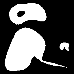
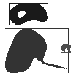
A function was created to do the object extraction.  It has two parameters: the number of objects and the binary image containing the objects. The algorithm works by first scanning the entire image until it hits an 'ON' pixel (level 1 if normalized).  Once such a pixel was found, that pixel was dilated with a structuring element B. The resulting dilation was intersected with the original image and then stored in a matrix V.  Upon each iteration, V was checked to see if it changed from the previous value of V.  If V did not change, the object was found and the algorithm stopped iterating. Thus, upon V reaching a steady state, the iterations stop.

B = 111
    111
    111

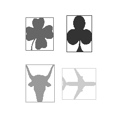
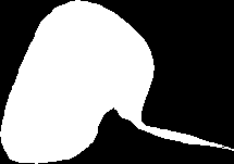
Next, the bounding box for the object recently found was computed. This was done by scanning the image V and determining the greatest and smallest values at which a ON pixel existed for both the X and Y axis.  It should be noted that the bounding box was constructed to INCLUDE the box itself as part of the image. Thus, the values computed for the top, bottom, left, and right of the object can be solely used without modification to quickly extract the object.  The box was drawn around the object using a for loop and is the same color as the image.

The images were colored such that they would be easily resolved as unique shades of gray to the human eye. This is why the number of objects was passed to the findObjects function. This enabled us to calculate the color values of each object before running the iterative algorithms described above. The found objects in their image were written out to disk with the appropriate color for identification.

The results of the object identification are shown below (Figures 4 - 6). Note that each object is a different shade of gray. The background of the image each of these objects are contained in is white

Figure 4: Three shapes extracted. (TheThreeShapes2_objects.png)	Figure 5: Nine letters extracted (penn256_objects.png)	Figure 6: Four distinct objects extracted. (match1_objects.gif)

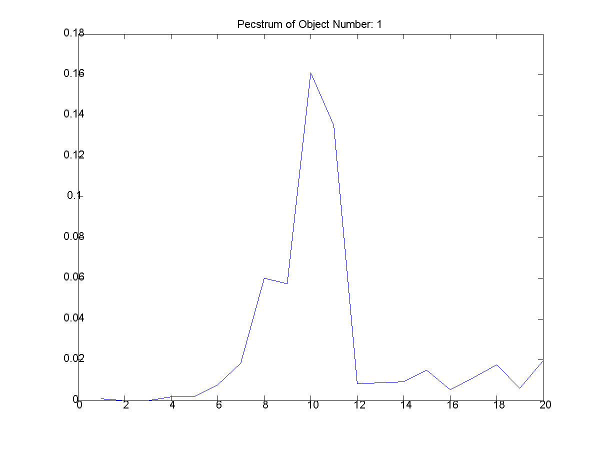
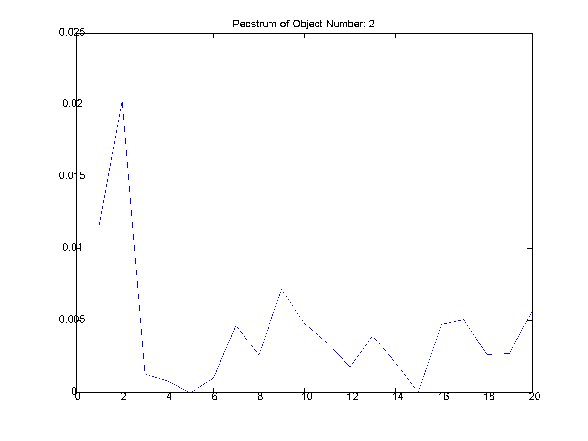
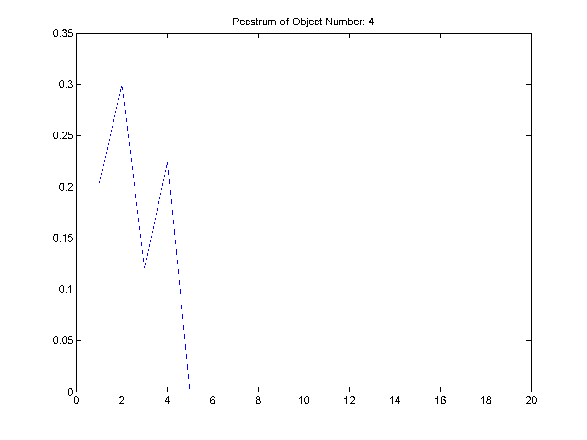
Upon completion of the bounding box,  the pecstrum of each object found in the input image was computed. The following algorithm was used to compute the pecstrum.

B = 111
    111
    111

pecstrum = f(n) = [ m(XnB) - m(X(n+1)B) ] / [m(X)]

          where m is the 'area' of the object.

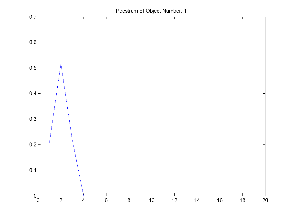
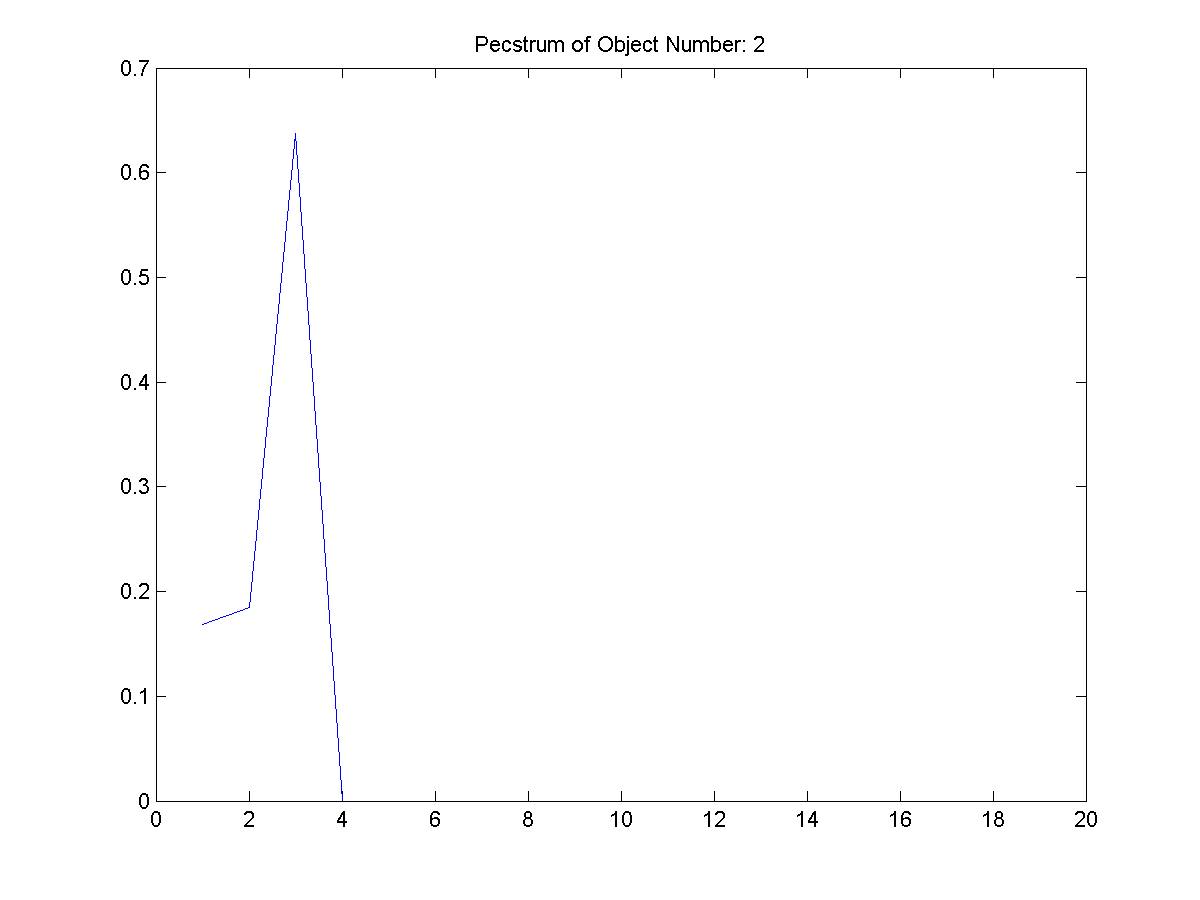
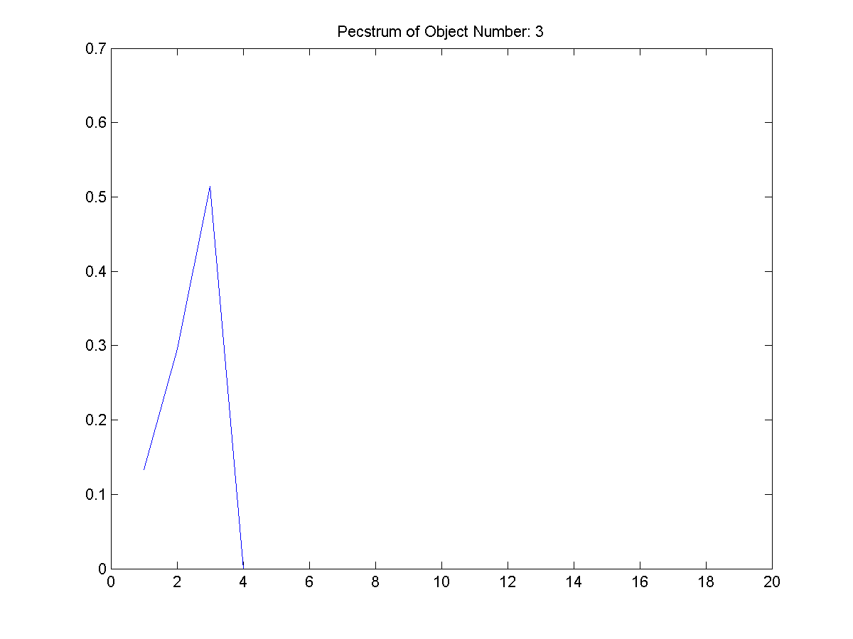
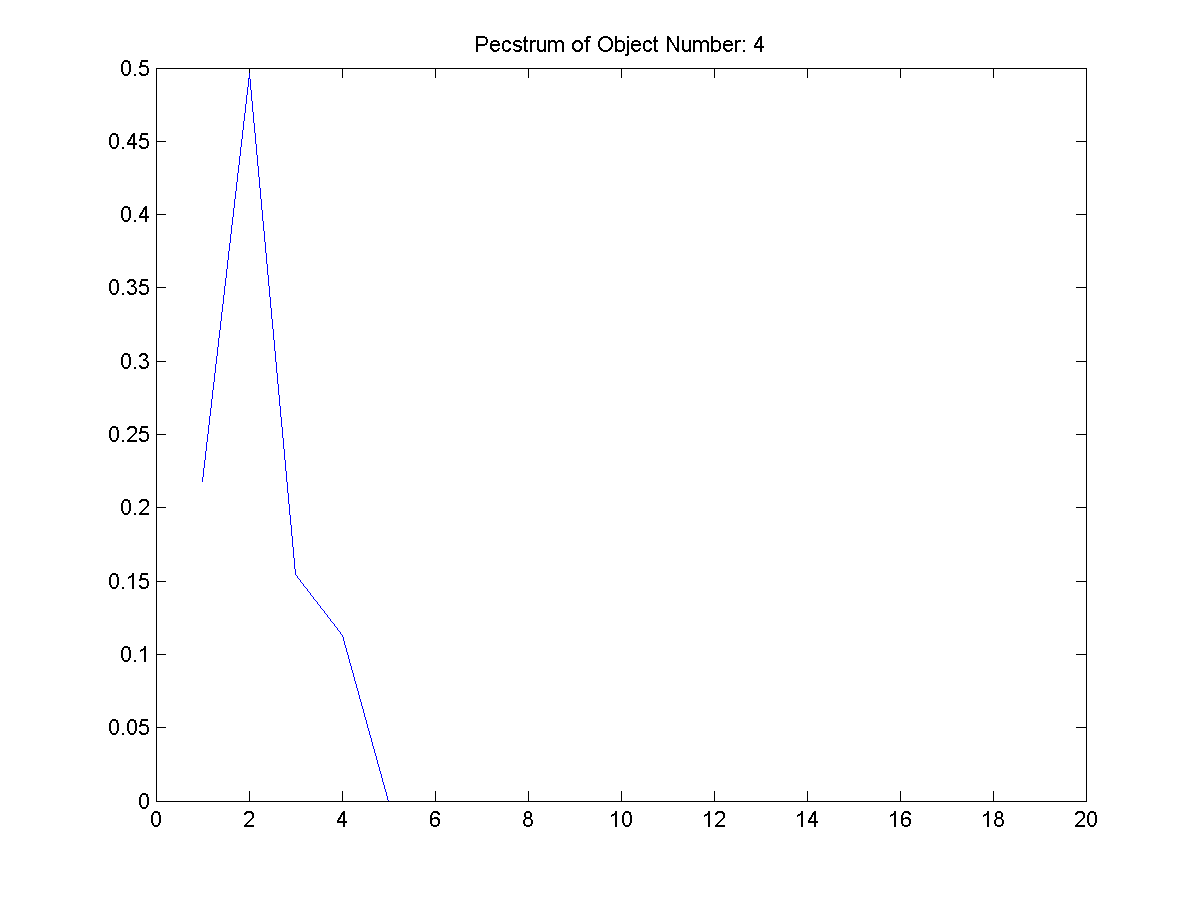
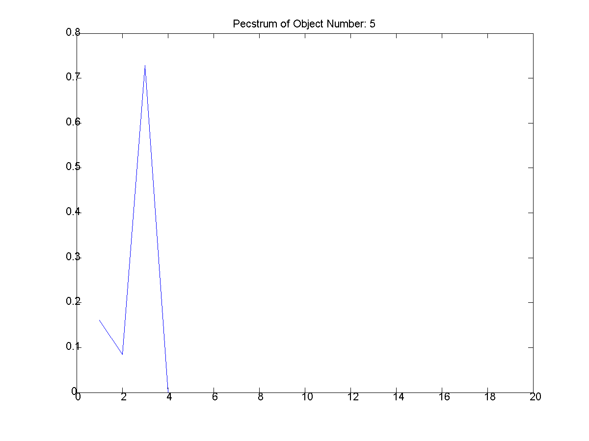
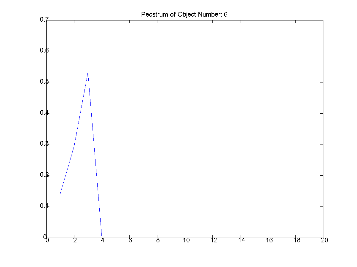
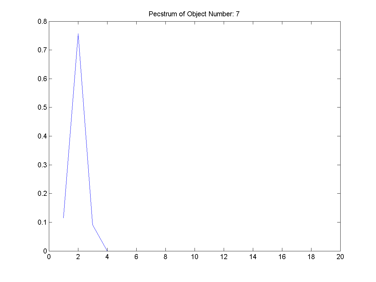
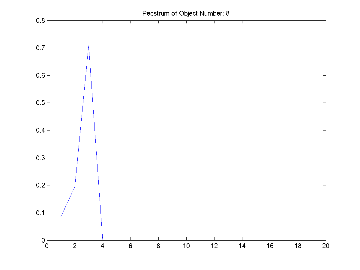
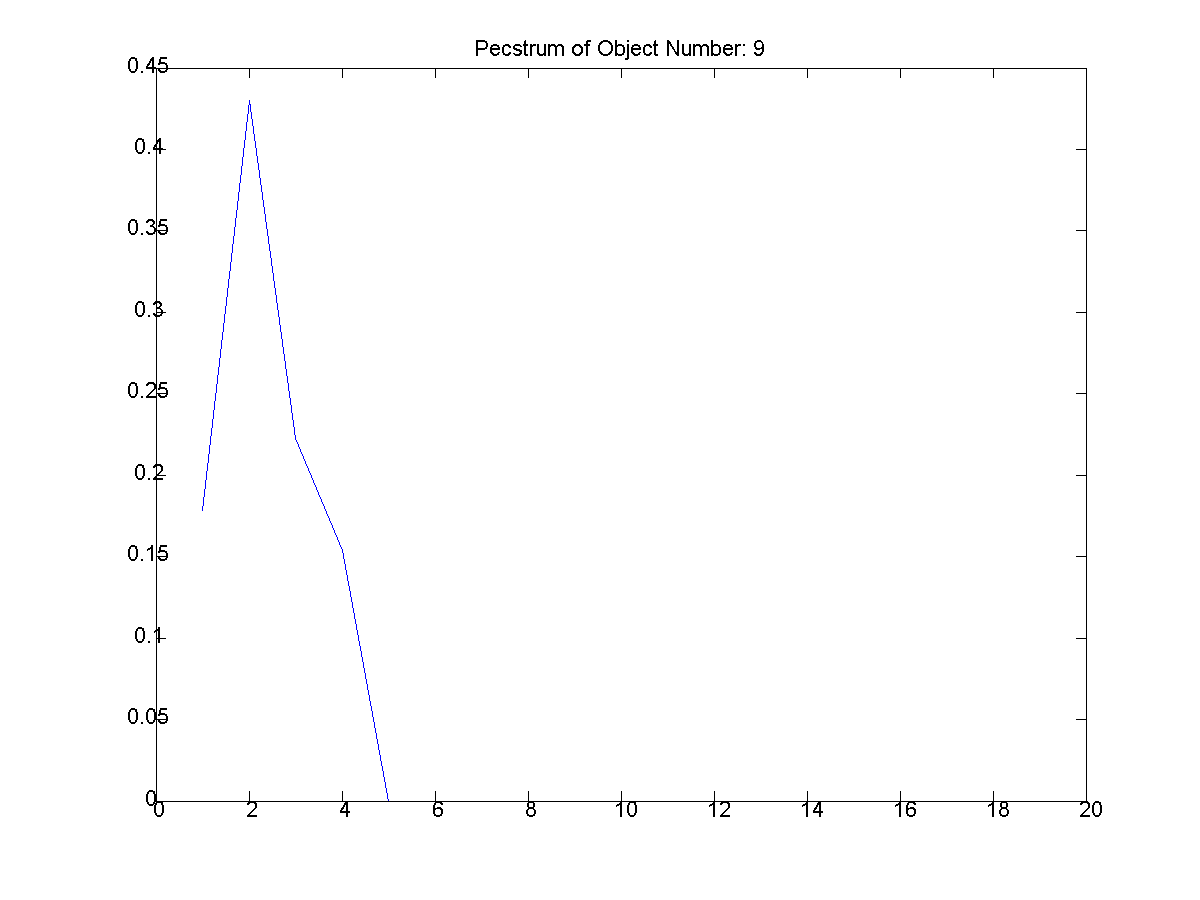
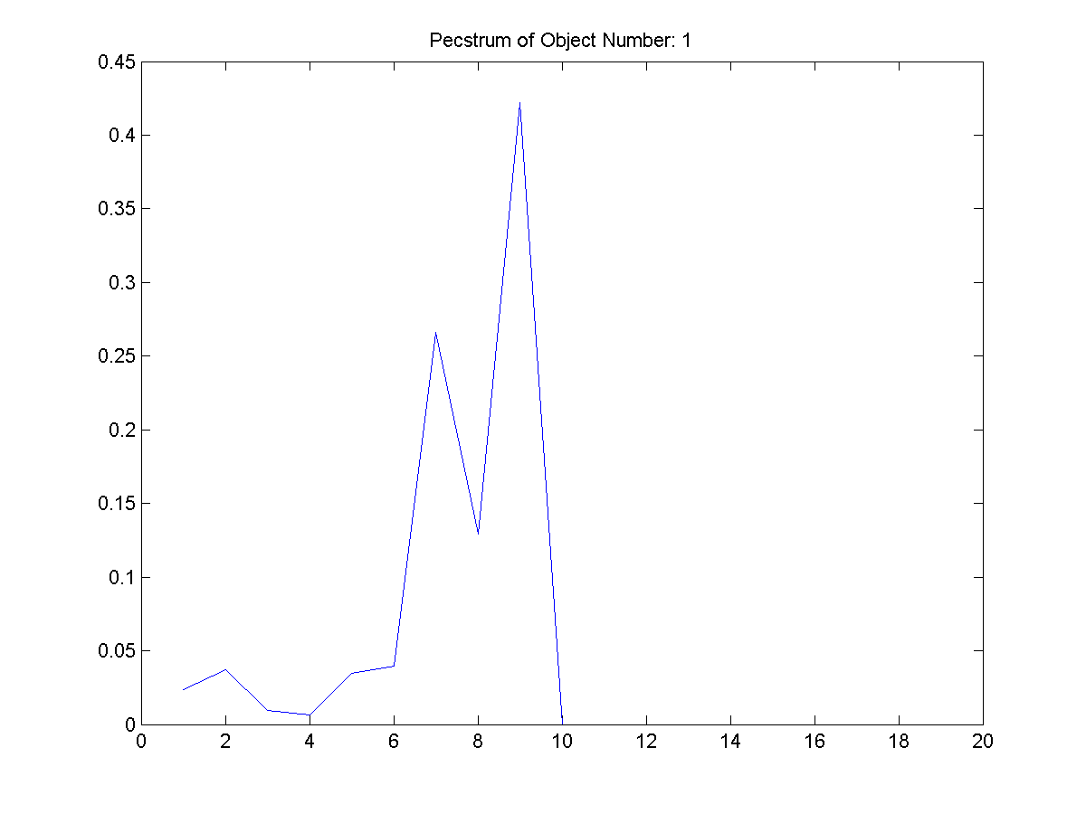
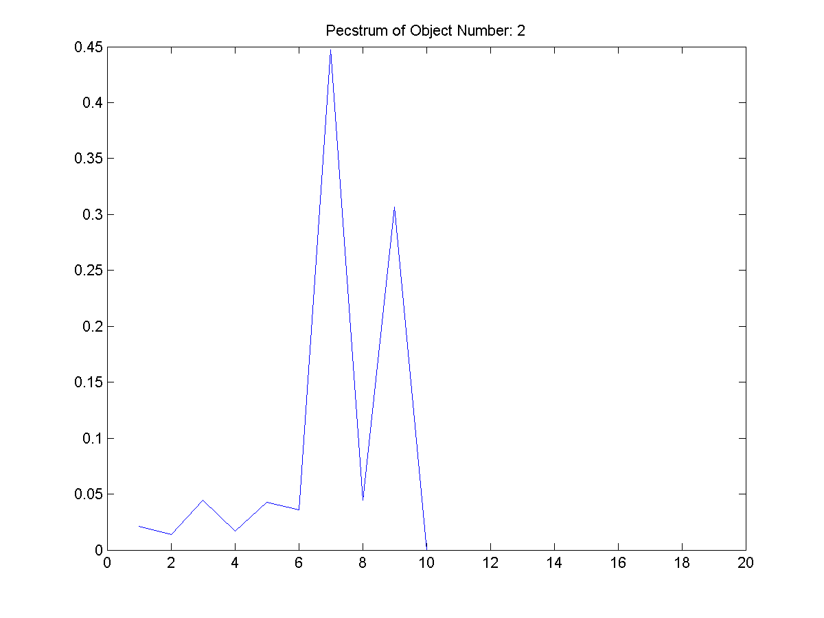
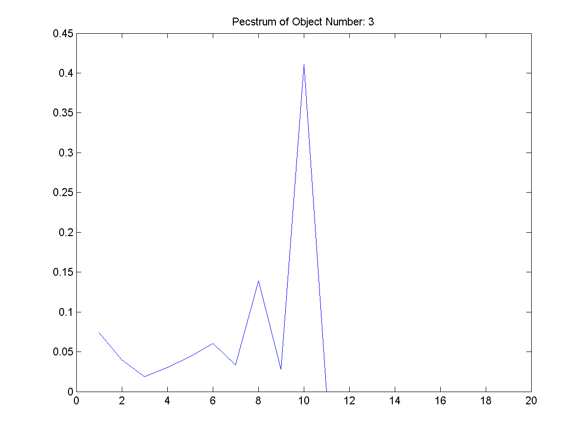
The results pecstrum of each object is shown below (Figures 7-22). Note that the domain of the pecstrum is discrete and not continuous as depicted by the MATLAB PLOT command. However, the values at each point in the discrete domain are correct.  Each pecstrum graph can be blown up by clicking on it.

From Figure 1, these three shapes were extracted. The first object filename is provided as the other are of similar pattern.

Figure 7: The first extracted object and its pecstrum below it. (T: thethreeshapes2/object_1.png, B:thethreeshapes2/object_1_pectsrum.png)	Figure 8: The second extracted object and its pecstrum below it.	Figure 9 The third extracted object and its pecstrum below it.

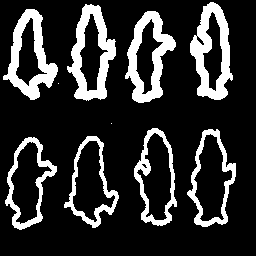
From Figure 2, these three shapes were extracted.  The table below represents Figures 10 -18.  Each extracted objects pecstrum is adjacent to itself.  The first object filename is provided as the other are of similar pattern.

(L:penn256/object_1.png,  R:penn256/object_1_pectsrum.png)

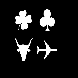
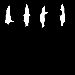
From Figure 3, these four shapes were extracted. The first object filename is provided as the other are of similar pattern.

Figure 19: The first extracted object and its pecstrum adjacent to it. (L: match1/object_1.png, match1/object_1_pectsrum.png)
Figure 20: The second extracted object and its pecstrum adjacent to it.
Figure 21: The third extracted object and its pecstrum adjacent to it.
Figure 22: The fourth extracted object and its pecstrum adjacent to it.

Part 1.B

The second section of Part 1, section b,  was to compute the pecstrums as shown above.  Figure 8, from its pecstrum, appears to be the most complex object extracted from the three images.  Its pecstrum has many delta functions implying the object is very "jaggy". Typically jaggy objects are not have little repetition (patterns) and symmetry and can be described as complex because so. Many of the other objects in the data set have straight edges or have symmetric properties. Thus, they are few deltas in their pecstrum.

Pecstrum is somewhat analogous to frequency spectrum. It should be noted that similar to a frequency spectrum, the sum of the area under each pecstrum function is equal to one. 

Part 2

This part of the project focused on morphological skeletonization. The process of skeletonization creates a set of skeletons for a given image.  Each skeleton represents a degree of detail in the original image. The skeletons are generated sequentially, with the first skeletongs Sk(0), Sk(1), etc. containing the smallest details in the original image.  The larger order skeletons Sk(n), Sk(n-1), etc. contain the "meat" of the objects in the original image. There are a variety of variables in skeletonization, including the way in which it is applied and the structuring element used to apply it. Generally, one would like to use a circular structuring element of relatively small radius with respect to the object.  In the discrete domain, however, the circle must be approximated and cannot be smaller that 5x5. This structuring element, shown as "B" below, was chosen for this part of the project, as recommended by Pitas and Venetsanopoulos.

B = 0 1 1 1 0
    1 1 1 1 1
    1 1 1 1 1
    1 1 1 1 1
    0 1 1 1 0



Part 2.A

The goal of this part is to implement and test the skeletonization algorithm on two test images. The images chosen are show in in figures 23 and 25. Results for each are in Figures 24 and 24 The algorithm implemented is document in P&V 6.8.7-6.8.10 and Figure 6.8.4 (a). The output of this routine is a large matrix of skeletons, Si(X), and the union of these. The latter output constitutes the morphological skeleton of the original image.

Figure 23: Original image (match1.gif)
Figure 24: Skeleton of match1.gif (match1skel.png)
Figure 25:Original image (bear.gif)
Figure 26: Skeleton of bear.gif (bearskel.png)

Comparing results to P&V Figure 6.8.4 it is clear that the algorithm performs as desired. Particularly remarkable effects are the generally irregular shape of the skeletons and preservation of the salt noise pixels in the bear image. The morphological skeletonization routine is clearly not perfect, but it achieves the desired result of finding the medial axis of objects. A subsequent operation that performs object connection and removes outliers would enhance the usefulness of the result.

Part 2.B

The goal of this part is to take the skeletons (S0(X), S1(X1), ..., SN(X)) from Part 2.A and attempt to partially reconstruct the original image. The reconstruction will be based on the "meat" of the image, that is SN(X), SN-1(X), SN-2(X) and SN-3(X). The alorithm used is documented in P&V 6.8.10 and Figure 6.8.5 (b). The routine that accomplishes the partial reconstruction accepts a large matrix of all skeletons, Si(X), and picks of the four largest. These are then feed through the algorithm. For comparision, a full reconstruction of bear.gif is provided to demonstrate the effectiveness of the reconstruction algorithm.

Figure 27: Partial reconstruction of the match1.gif skeleton (matchrecon.png)
Figure 28: Set difference between skeleton of match1.gif and partial reconstruction (matchrecon_diff.png)
Figure 29: Partial reconstruction of the bear.gif skeleton (bearrecon.png)
Figure 30 Set difference between skeleton of bear.gif and partial reconstruction (bearrecon_diff.png)
Figure 31: Full reconstruction of the bear.gif skeleton (bearrecon_FULL.png)
Figure 32: Set difference between skeleton of bear.gif and full reconstruction (bearrecon_FULL_diff.png)

It is clear from the results in Figures 27 and 29 that the partial reconstruction using only the four highest order skeletal components removes details. This is clearly realized when examining the partial reconstruction resutls for bear.gif and realizing that the "outline bears" are completely removed. Since the outlines are relatively thin, they are not present in the four highest order skeletal components.  Note that if the outlines had been the only thing present in the image (the solid bears were absent) they would be present in the partial reconstruction as the highest order skeletal components would not be as high order as those requried to skeletonize the solid bears. Finally, observing the results in Figures 31 and 32 one can see that the skeletonization algorithm allows perfect reconstruction of the original image if all skeletal components are used (this is shown because the set difference between the full reconstruction and the original image is zero).

Part 2.C

All results and figures for Part 2 are given and discussed in their respective sections (A or B) above.

Summary

The results presented here are relatively straight forward. All outcomes achieved were as expected in each experiment, as we were able to predict what we should see and explain each result.  Practical uses and analysis of  basic morphological operations and algorithms are demonstrated.

D.

Conclusions

Conditional dilation is a great way to extract separate object or components from a binary image. It is not the speediest of algorithms but yet accomplishes the job well doing no extra that what is minimal needed. The algorithm could be sped up by using a very specialized hit-or-miss transform with a suitable structuring element. However, this may not be robust enough to work efficiently for all scenarios.  

The pattern spectrum, or simply pecstrum, it a way to measure pattern content of a binary image or object.  Its useful in associating a function to image complexity or jaggedness.  The pecstrum is a very important function with many uses including binary pattern recognition. 

Morphological skeletonization does not produce pristine skeletons.  It does, however, accomplish the desired operation of skeletonization in that the original image can be successfully reconstructed from its skeleton. Each skeleton also contains the progressively increasing degree of detail that is desired. The algorithm provided by Pitas and Venetsanopoulos (taken from Maragos) is relatively easy to implement and performs well.

E.

Appendix

This appendix contains the source code for our project. The code is shown below in a way that reflects the hierarchy of dependencies. Please refer to the comments at the top of each function for a complete description.

• findObjects.m
  • erosion.m
    • erode.m
  • dilation.m
  • setdifference.m
  • intersection.m
  • area.m
• skeleton.m
  • SK.m
    • erosion.m
      • erode.m
    • dilation.m
    • setdifference.m
  • dilation.m
  • setdifference.m
  • union.m