A.

 Objectives

1. Become familiar with grayscale filtering techniques including symmetric nearest-neighbor mean, Close-Open, 2D median, and anisotropic diffusion.
2. Study how different filters compare to each other in terms of remove noise, preserving edgets, etc.
3. Study filter properties such as median roots.
4. Become familer with interpreting histograms to segment images from different filtering methods.
5. Learn when to use what filter and why in a noisy situation.
6. Study how different variables and equations affect the performance of a filter, particularly anisotropic diffusion.
7. Discuss how the filter methods described above can be applied to real-world applications.
8. Explore several different order statistic operations and compare them to the morphological close-open operation.
9. Observe the effects of repeated application of several algorithms.
10. Evaluate the performance of algorithms as they approach a root.
11. Evaluate the performance of algorithms on different types of images.

B.

Methods

The experiment was written in terms of many MATLAB functions with no single script used to execute the entire experiment.  The functions below were executed at the command line to generate the results.  Each function is described below.

atdiffusion.m  (atdiffusion function)

The function performs anisotropic diffusion on an input image.  It uses a specified equation for diffusion along with a lambda of 0.25.  The function can also perform the filter over many iterations as specified by the user. A grayscale image with the filter iteratively applied is return.

snnm.m (snnm function)

This function performs 7x7 symmetric nearest-neighbor mean filter on a grayscale image.  The filtered image is returned.

alphamean.m (alphamean function)

This function performs alpha-trimmed mean filtering using the specified window size and "trim" factors.  A filtered image is returned.

dilation.m & erosion.m (dilation and erosion functions respectively)

Our previous dilation and erosion operators were slightly modified in order to properly handle grayscale images.

Executing the functions from MATLAB

Please see the associated help with function. At the command prompt type:

>>help functionname

C.

Results

Part 1

This part of the project focused on the effects of repeated application of several algorithms. The results were observed in the form of image output and by obtaining the histogram of the image. All of the algorithms considered are implemented for use on grayscale images.

Part 1.A

The algorithms developed and a brief description of each is given:

• 7x7 Median -- the median operation preserves edges while doing a good job of removing outliers (which are details that are very small relative to the size of the mask).
• 7x7 Alpha-Trimmed Mean -- this operation finds the mean of the points in a mask exclusing those that are much larger or much smaller than the median. Performing this operation requires sorting the data.
• 7x7 Symmetric Nearest Neighbor Mean -- this algorithm operates on the pixels within its mask in pairs, comparing each pair of pixels to the center pixel and keeping only those that are "most similar."
• 3x3 Morphological Close-Open -- this operation is useful for removing small artifacts (cavities, etc.).

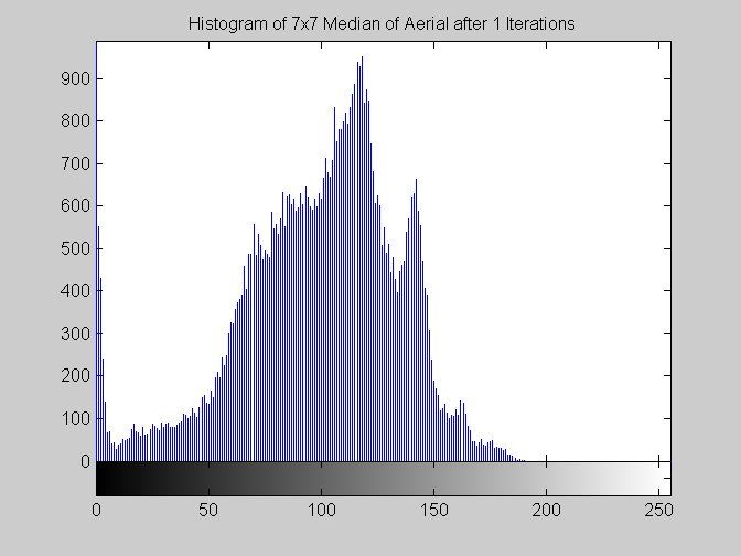
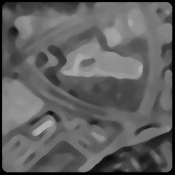
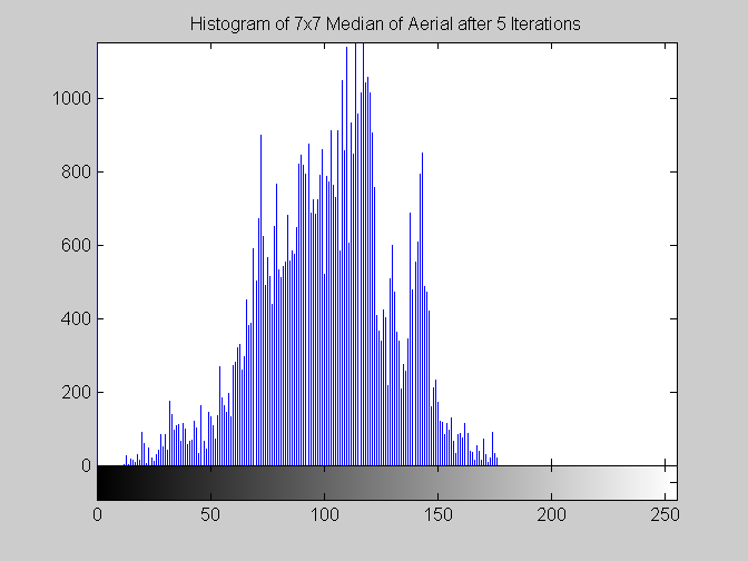
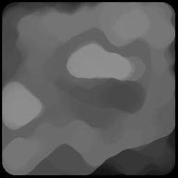
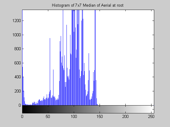
Part 1.B

Each algorithm was applied to aerial.gif and disk.gif. Results are observed after one and five iterations as well as after a root is reached. Some algorithms seemed to be taking an enormous amount of time to reach a root. In these cases the root was approximated by a large number of iterations (approximately 100). When this approximation is made comments are given that indicate what the root of the algorithm would be, based on the observed results at a large number of iterations. This approach was used at the suggestion of Dr. Higgins in lecture.

7x7 Median Filter (aerial.gif)

Figure 1: Original image (aerial.gif)
Figure 2: One iteration
Figure 3: Histogram
Figure 4: 5 iterations
Figure 5: Histogram
Figure 6: Root (estimated at 130 iterations)
Figure 7: Histogram

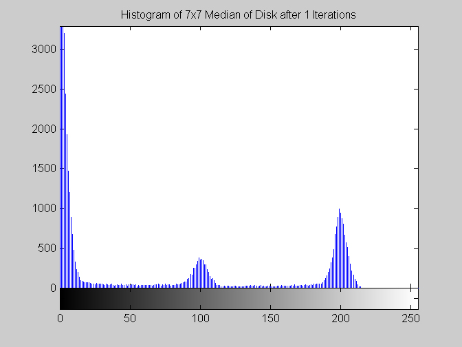
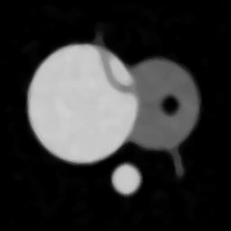
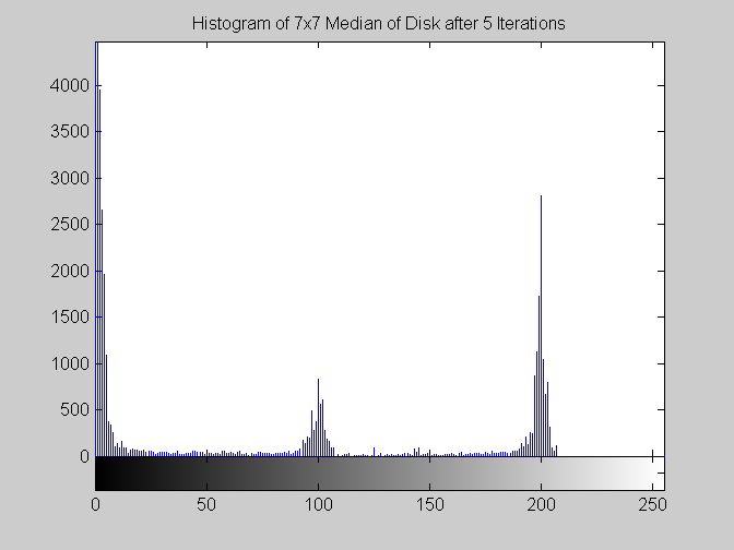
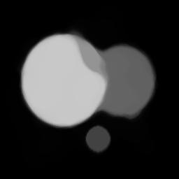
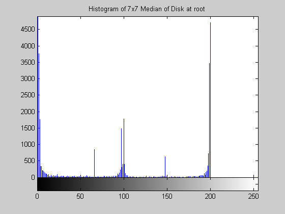
7x7 Median Filter (disk.gif)

Figure 1: Original image (disk.gif)
Figure 2: One iteration
Figure 3: Histogram
Figure 4: 5 iterations
Figure 5: Histogram
Figure 6: Root (estimated at 105 iterations)
Figure 7: Histogram

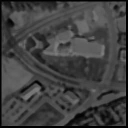
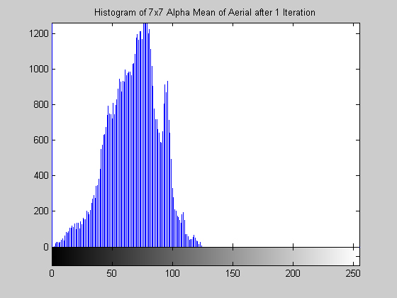
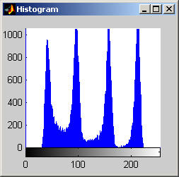
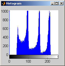
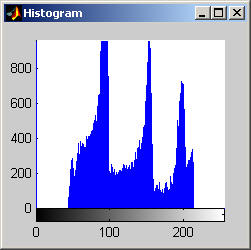
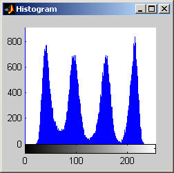
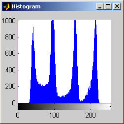
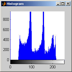
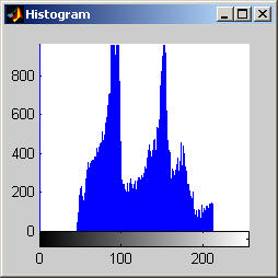
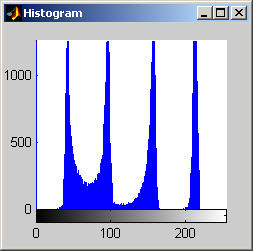
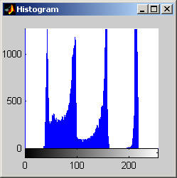
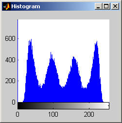
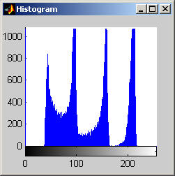
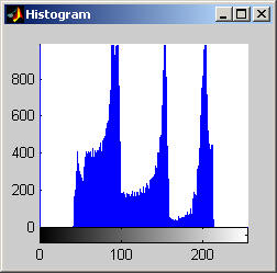
It is worth mentioning, with the presentation of these first results, that each filter in this project presented had local knowledge problem as a result of the finite images used to test their operation. The problem was solved by excluding calculation for pixels which could not support the mask completely.  Therefore, for filters with a 7x7 mask (like the median discussed directly below) a border of 3 pixels on all sides of the image is excluded from calculation (no result is obtained for these pixels and they are set to zero, appearing black in the results presented).  One can observe that repeated application of the filter causes this local knowledge problem to creep into the image, particularly at the corners.  It is assumed that the results around the edges are not exactly correct but that the bulk of the results, contained in the middle of the image (say 245x245 pixels at the minimum), are correct.

The results show that the median filter is edge preserving, at least to the extent that the edges present are large enough not to be treated as small details.  The median filter is very good at removing salt and pepper noise, as evidenced by the results on the disk image.  However, this same behavior serves to annihilate (potentially useful) details in the aerial image. The first iteration of the median algorithm has remarkable effects on the aerial image (small details are immediately removed), while the results on the disk image are not quite as noteworthy. By the fifth iteration the behavior the median filter is quite clear -- the noise in the disk image is already largely removed.

As a root is approached very few graylevels remain.  Looking at the histograms for the disk image as the number of iterations increases it can be seen that several discrete graylevel values are being approached. Interestingly, the cavity in one circle is filled in while a small object of nearly the same size remains. Presumably, at the root, the three major gray level values for each of the three objects in the disk image would be all that is remaining. Because the aerial image is much more complicated, it is difficult to see the same trend as clearly in its histograms. However, as the number of iterations increases, large peaks certainly begin to form implying that the same effect will be achieved, though it seems it may take even more iterations to reach it.

7x7 Alpha-Trimmed Mean Filter (aerial.gif)

Figure 1: Original image (aerial.gif)
Figure 2: One iteration
Figure 3: Histogram
Figure 4: 5 iterations
Figure 5: Histogram
Figure 6: Root (found at 15 iterations)
Figure 7: Histogram

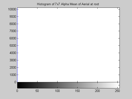
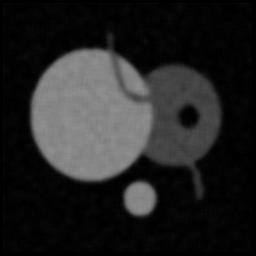
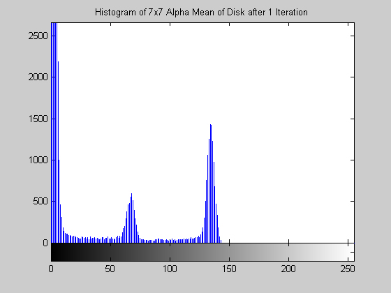
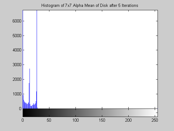
7x7 Alpha-Trimmed Mean Filter (disk.gif)

Figure 1: Original image (disk.gif)
Figure 2: One iteration
Figure 3: Histogram
Figure 4: 5 iterations
Figure 5: Histogram
Figure 6: Root (found at 15 iterations)
Figure 7: Histogram

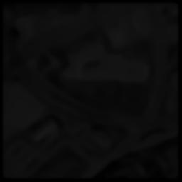
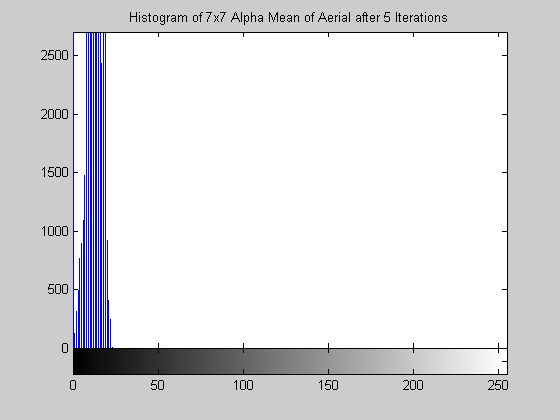
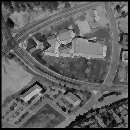
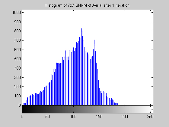
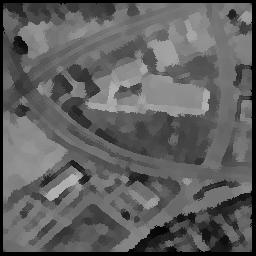
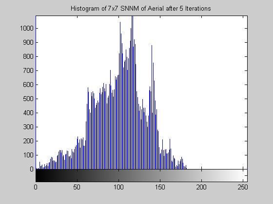
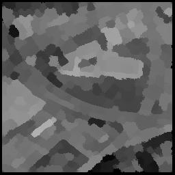
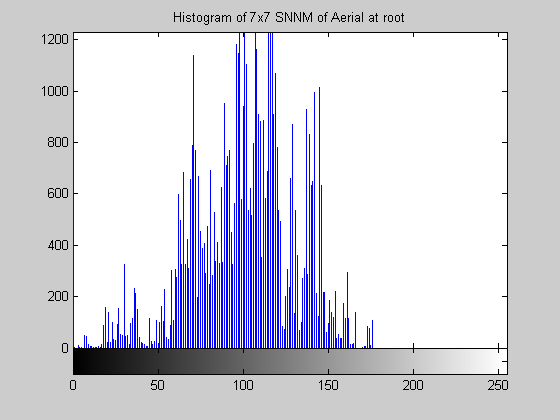
The effect of this filter is quite interesting. Examining the results in the form of an image is not too telling, the image appears to simply be darkened by operation. However, the operation has compressed the histogram while preserving its shape.  This can been seen very clearly for the disk image, the three prominent gray levels remain but are pushed ever closer to 0. The aerial image produces similar results.  This algorithm also approaches a root relatively quickly, by 15 iterations the histogram is compressed completely to zero.

7x7 Symmetric Nearest Neighbor Mean Filter (aerial.gif)

Figure 1: Original image (aerial.gif)
Figure 2: One iteration
Figure 3: Histogram
Figure 4: 5 iterations
Figure 5: Histogram
Figure 6: Root (estimated at 105 iterations)
Figure 7: Histogram

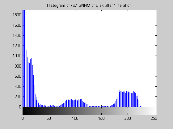
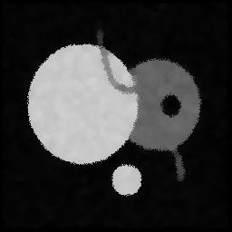
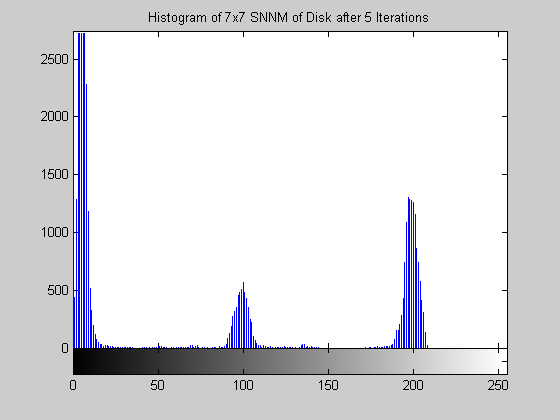
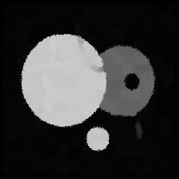
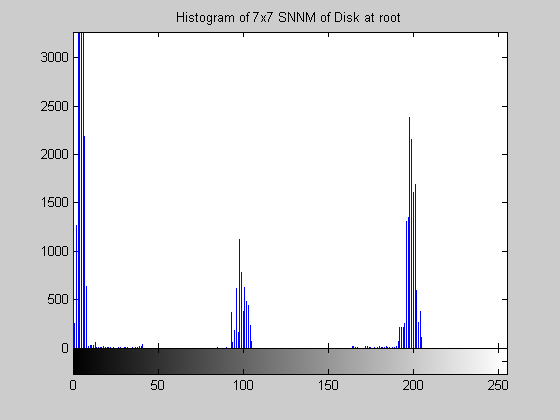
7x7 Symmetric Nearest Neighbor Mean Filter (disk.gif)

Figure 1: Original image (disk.gif)
Figure 2: One iteration
Figure 3: Histogram
Figure 4: 5 iterations
Figure 5: Histogram
Figure 6: Root (estimated at 105 iterations)
Figure 7: Histogram

This algorithm yields a result that is similar to that of the median, but is it much less aggressive. The algorithm does a fairly good job at removing salt and pepper noise, as the images and histograms reveal for the disk image. The final results appear "blotchy" which is shown in the histograms by groups of gray levels remaining accented.  The algorithm seems to be preserving ranges of gray levels rather than selecting a single to highlight. The results from the aerial image are particularly remarkable, especially when compared to the median filter.  Though small details are still removed, may of the objects in the image are "preserved" in the sense that a connected region of a nearly single gray level remains to represent the object. The road and other large structures are still readily obvious even after 105 iterations (nearly a root). This result implies that the SNNM would be well suited for a crude segmentation algorithm.

Close-Open Filter (aerial.gif)

Figure 1: Original image (aerial.gif)
Figure 2: One iteration
Figure 3: Histogram
Figure 4: 5 iterations (also a root)
Figure 5: Histogram

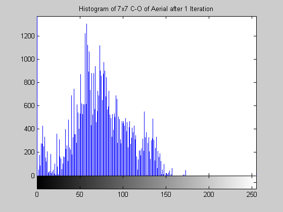
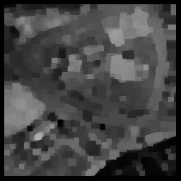
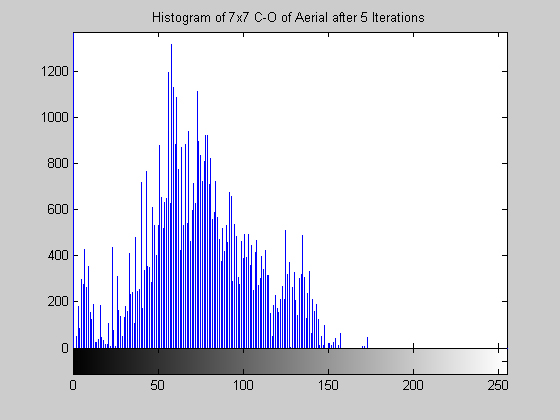
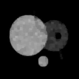
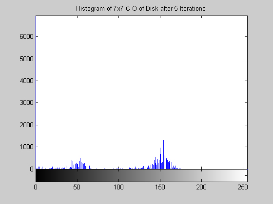
Close-Open Filter (disk.gif)

Figure 1: Original image (disk.gif)
Figure 2: One iteration
Figure 3: Histogram
Figure 4: 5 iterations (also a root)
Figure 5: Histogram

The morphological close-open operation is idempotent. Therefore, after even just five iterations, the result is no longer changing. Visually comparing the resultant images for one and five iterations and their accompanying histograms it is clear the subsequent applications had no effect.

Morphological filters do not handle salt and pepper noise well.  This is exemplified by the results for the disk image. One can also note that for the disk image the histograms appear "small" -- there is a really large concentration of points at 0 that makes the rest of the graylevel values seems small in comparision. For this image the close-open operation has drastically reduced the average gray level of the image. The same effect is not apparent in the aerial image. This image does, however, show that the close-open does not perform much of an organized operation on the histogram. No peaks are accentuated at any particular graylevels or groups of graylevels.

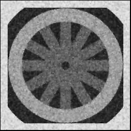
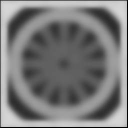
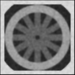
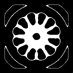
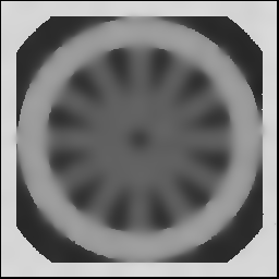
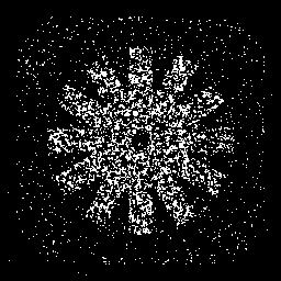
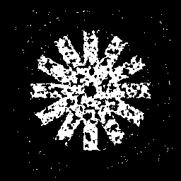
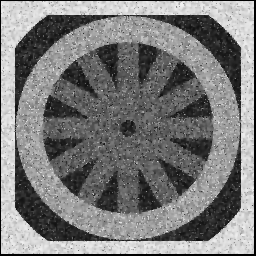
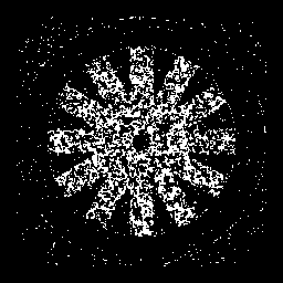
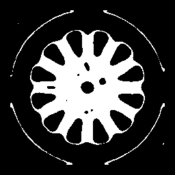
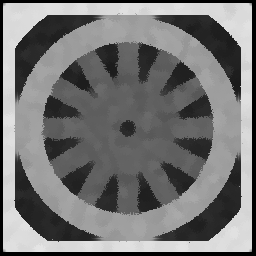
Part 2.a

The results for each iterations are stacked vertically.  In the segmented image sections, we are attempting to best extract the spokes of the wheel. Each image has a plot of its horizontal cross section at y=128.  Each image is not specifically labels, however, the images are in a table for easy comparison.

Original Image wheeln40.gif
g( ) = Exponential function K = 50 Lambda = 0.25
5 Iterations	15 Iterations	50 Iterations	100 Iterations
Histograms
Sample at y = 128
Segmented Image - Grayscales(80 -110)	(80 - 110)	(80 - 110)	(90 - 100)
g( ) = Quadratic function K = 50 Lambda = 0.25
5 Iterations	15 Iterations	50 Iterations	100 Iterations
Histograms
Sample at y = 128
Segmented Image - Grayscales(80 -110)	(80 -110)	(90 -105)	(90 - 105)
The anisotropic diffusion works well at low iterations in removing some of the noise. However, as the iterations increase, the image becomes more blurry than anything else. This is especially visible in the cross sections of each image at y=128.  This fact makes image segmentation much harder as the gray level tend to mesh together to a constant.  This is shown in the segmented images as with the higher iterations, the spokes are harder to isolate.  With few iterations, the spokes still have visible noise in them which affects the image segmentation preventing a solid image of the spokes to be realized correctly. The use of g( ) as an exponential yields preservation of high contrast, large gradient edges in each iterations.  There is less blurry and "leakage" at the edges of the spokes and rubber with the exponential.  The use of g( ) as a quadratic really favors the large areas of one shade of gray. These areas are much better preserved over many iterations. This fact is especially apparent with the segmented images as the spokes are better resolved at the edges with the exponential rather than the quadratic.  This fact is also displayed in the histograms as there appears to be more "peakiness" in the histograms using the exponential and not the quadratic.  In all images, the profile tends to near a constant as the number of iterations goes up. This is expected as with such a large "blurrying" factor, K=50, the images quickly become blurry with lots of iterations and eventually, all detail is lost.
g( ) = Exponential function K = 25 Lambda = 0.25
5 Iterations	15 Iterations	50 Iterations	100 Iterations
Histograms
Sample at y = 128
Segmented Image - Grayscales(80 -110)	(80-100)	(80-100)	(80-100)
g( ) = Quadratic function K = 25 Lambda = 0.25
5 Iterations	15 Iterations	50 Iterations	100 Iterations
Histograms
Sample at y = 128
Segmented Image - Grayscales(80 -110)	(80-100)	(80-100)	(80-100)
The lower K value, K=25, used to generate these images seems to make the results much more usable as far as segmenting goes. The images tend not to blur as much as the iterations increase.  In fact, K=25 is very good at preserving the edges throughout the iterations and does a fair job at removing noise and restoring the original, noiseless image.  The exponential used for the first set of images shows this preservation of details in the histograms.  These histograms have very high peaks with little surrounding noise when compared to the quadratic. It appears that K controls the amount of diffusion the noise is spread throughout the image.  The edges are preserved very well when using the exponential.  However, the quadratic is much better at removing noise from large blobs of gray color.

 

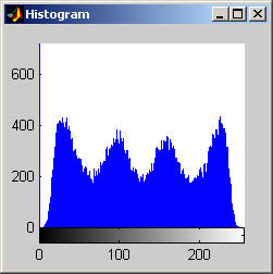
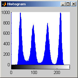
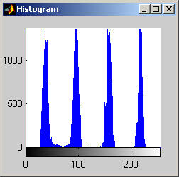
Part 2.b

10 iterations of the 7x7 symmetric nearest-neighbor mean filter yields the following data:

Filtered Image	Histogram	Sample at y = 128	Segmented Image (90-105)

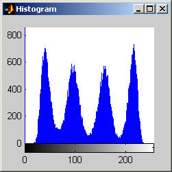
As shown above, the 7x7 symmetric nearest-neighbor mean (SNNM) filter dos not blur the noise into the image as much as anisotropic diffusion.  This fact is espeically visible with high iterations of anisotropic diffusion.  The SNNM filter tends to better reach the true values (peaks in the histogram) of the image quicker and more accurately than the anisotropic diffusion filter.  Of all the filters inspected, the SNNM yeilding the most "peaky" histogram.  Better peaks are visible in the SNNM filtered image's histogram and thus making segmentation results much better as shown.

Part 2.c

Original Image aerial.gif		Sample at y = 128 or aerial.gif
g( ) = Exponential function K = 50 Lambda = 0.25
5 Iterations	15 Iterations	50 Iterations	100 Iterations
Sample at y = 128
g( ) = Quadratic function K = 50 Lambda = 0.25
5 Iterations	15 Iterations	50 Iterations	100 Iterations
Sample at y = 128

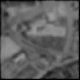
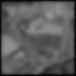
As demonstrated with the wheel image, the quadratic tends to better preserve large blobs of color and the exponential better preserves edges and details. This difference is very apparent if you inspect the large buildings in the center of the images. The edges of the roofs are much clearing when using the exponential than with the quadratic. However, with the quadratic, it is easier to resolve sweeping features such as the entire roof and the roads and other different land vegetation.  This is because the quadratic excels at preserving the large blobs which in aerial images are usually large roads and vegetation as they sweep far across the land.

In all the tests run, as the iteration increases the images appear to approach a mean value, the noise is smeared around so much at high iterations that little detail can be made out and sweeping blobs of a few shades dominate the image.

 

D.

Conclusions

Anisotropic diffusion is great at removing noise for low iterations.  At high iterations, the "diffusion" functions dominate the image and the image appears to approach a mean as details is lost.  The quadratic function used in the diffusion is better at persevering large blobs of gray as opposed to the exponential function which tends to better preserve edges and detail.  However, at large iterations, both functions cause the diffusion to blur causing lost of detail. As we increase K, the amount of "smearing" increases greatly. A more modest value of K however produces great results that are useful in segmenting out parts of an image as they create a better "peakiness" in the image's histogram.

The SNNM filter is also great at low iterations in cleaning up grayscale images with few colors and lots of noise.  With only a few iterations, the grayscale values tend to attract to peaks in the histogram thereby making segmentation a much easier job to perform.  The SNNM results in the highest "peakiness" among values in all the histograms created.

The anisotropic diffusion is not well suited to extract details from a complex scene unless one is looking for sweeping generalizations in the image.  In the wheel image, the diffusion was great at removing noise and preserving the pieces of the wheel and even better defining them.  However, in the case of the aerial image, with many iterations, only dominating blobs of gray were well preserved.  The aerial image is too complex to produce great segmentation of things such as a small rooftop, etc.  However, the details in the wheel were still well preserved at low iterations and useful in segmenting.  It should be noted though that the details in the aerial image were will preserved at low iterations, making it a good choice to use when segmenting a scene by vegetation, agriculture, etc.  The building also were much more apparent when using the exponential making it a possible choice for detail extraction.

E.

Appendix

This appendix contains the source code for our project. The code is shown below in a way that reflects the hierarchy of dependencies. Please refer to the comments at the top of each function for a complete description.

• alphamean.m
• dilation.m
• erosion.m
• median.m
• snnm.m

atdiffusion.m
snnm.m